5.4 In-Class Exercises
In these exercises, we’ll continue the factor analysis of the ESS data that we started in the At-Home Exercises.
5.4.1 Basic CFA
5.4.1.1
Load the ESS data.
- The relevant data are contained in the ess_round1.rds file.
We are going to extend our existing three-factor CFA by adding the five-factor representation of the Attitudes toward Immigration items suggested by Kestilä (2006). The hypothesized factor-to-item mapping is given below.
Trust in Institutions
trstlgl: Trust in the legal systemtrstplc: Trust in the policetrstun: Trust in the United Nationstrustep: Trust in the European Parliamenttrustprl: Trust in country’s parliament
Satisfaction with the Political Situation
stfhlth: State of health services in country nowadaysstfedu: State of education in country nowadaysstfeco: How satisfied with present state of economy in countrystfgov: How satisfied with the national governmentstfdem: How satisfied with the way democracy works in country
Trust in Politicians
pltinvt: Politicians interested in votes rather than peoples opinionspltcare: Politicians in general care what people like respondent thinktrstplt: Trust in politicians
Immigration Policy
imrcntr: Allow many/few immigrants from richer countries outside Europeeimrcnt: Allow many/few immigrants from richer countries in Europeeimpcnt: Allow many/few immigrants from poorer countries in Europeimsmetn: Allow many/few immigrants of same race/ethnic group as majorityimpcntr: Allow many/few immigrants from poorer countries outside Europeimdfetn: Allow many/few immigrants of different race/ethnic group from majority
Social Threat
imbgeco: Immigration bad or good for country’s economyimbleco: Taxes and services: immigrants take out more than they put in or lessimwbcnt: Immigrants make country worse or better place to liveimwbcrm: Immigrants make country’s crime problems worse or betterimtcjob: Immigrants take jobs away in country or create new jobsimueclt: Country’s cultural life undermined or enriched by immigrants
Refugee Policy
gvrfgap: Government should be generous judging applications for refugee statusimrsprc: Richer countries should be responsible for accepting people from poorer countriesrfgbfml: Granted refugees should be entitled to bring close family membersrfggvfn: Financial support to refugee applicants while cases consideredrfgawrk: People applying refugee status allowed to work while cases consideredrfgfrpc: Most refugee applicants not in real fear of persecution own countriesshrrfg: Country has more than its fair share of people applying refugee status
Cultural Threat
qfimchr: Qualification for immigration: christian backgroundqfimwht: Qualification for immigration: be whitepplstrd: Better for a country if almost everyone share customs and traditionsvrtrlg: Better for a country if a variety of different religions
Economic Threat
imwgdwn: Average wages/salaries generally brought down by immigrantsimhecop: Immigrants harm economic prospects of the poor more than the rich
5.4.1.2
Calculate the following quantities for the CFA described above.
- The number of model parameters
- The pieces of available information provided by the data
- The degrees of freedom after sufficiently identifying the model
Assume:
- Simple structure with no cross-loadings
- Enough constraints to locally identify each construct
- No mean structure
Click to show answer
Our model will have 38 observed indicators and 8 latent constructs, so we get the following values.
Model Parameters
- 8 (8 - 1) / 2 = 28 latent covariances
- 8 latent variances
- 38 factor loadings
- 38 residual variances
Total = 28 + 8 + 2 \(\times\) 38 = 112
Available Information
38 (38 + 1) / 2 = 741
Degrees of Freedom
To identify the model, we need to constrain one parameter in each construct’s sub-model. We also need to constrain another parameter in the sub-model for Economic Threat, because that construct has only two indicators. So, we need to constrain 9 parameters.
df = 741 - 112 + 9 = 638
5.4.1.3
Define the lavaan model syntax for the CFA described above.
- Enforce a simple structure: do not allow any cross-loadings.
- Covary all latent factors.
- Do not specify any mean structure.
- Save this model syntax as an object in your environment.
Click to show code
mod_trust_att <- '
## Trust in Institutions:
inst =~ trstlgl + trstplc + trstun + trstep + trstprl

## Satisfaction with the Political Situation:
sat =~ stfhlth + stfedu  + stfeco + stfgov + stfdem

## Trust in Politicians:
pol =~ pltinvt + pltcare + trstplt

## Immigration Policy:
immi =~ imrcntr + eimrcnt + eimpcnt + imsmetn + impcntr + imdfetn

## Social Threat:
social =~ imbgeco + imbleco + imwbcnt + imwbcrm + imtcjob + imueclt

## Refugee Policy:
refugee =~ gvrfgap + imrsprc + rfgbfml + rfggvfn + rfgawrk + rfgfrpc + shrrfg

## Cultural Threat:
cult =~ qfimchr + qfimwht + pplstrd + vrtrlg

## Economic Threat:
econ =~ l*imwgdwn + l*imhecop
'
Note: We equate the factor loadings for the Economic Threat factor because that construct is under-identified without the extra constraints.
5.4.1.4
Estimate the CFA model you defined above, and summarize the results.
- Use the
lavaan::cfa()function to estimate the model. - Use the fixed-factor method of identification
- Use the default settings for the
cfa()function. - Request the model fit statistics and standardized parameter estimates by specifying
fit.measures = TRUEandstandardized = TRUEinsummary().
Click to show code
## Load the lavaan package:
library(lavaan)

## Estimate the CFA model:
out_trust_att <- cfa(mod_trust_att, data = ess, std.lv = TRUE)

## Summarize the fitted model:
summary(out_trust_att, fit.measures = TRUE, standardized = TRUE)
## lavaan 0.6-19 ended normally after 55 iterations
##
## Estimator ML
## Optimization method NLMINB
## Number of model parameters 104
## Number of equality constraints 1
##
## Used Total
## Number of observations 11716 19690
##
## Model Test User Model:
##
## Test statistic 27329.813
## Degrees of freedom 638
## P-value (Chi-square) 0.000
##
## Model Test Baseline Model:
##
## Test statistic 201900.916
## Degrees of freedom 703
## P-value 0.000
##
## User Model versus Baseline Model:
##
## Comparative Fit Index (CFI) 0.867
## Tucker-Lewis Index (TLI) 0.854
##
## Loglikelihood and Information Criteria:
##
## Loglikelihood user model (H0) -715042.663
## Loglikelihood unrestricted model (H1) -701377.756
##
## Akaike (AIC) 1430291.326
## Bayesian (BIC) 1431050.303
## Sample-size adjusted Bayesian (SABIC) 1430722.981
##
## Root Mean Square Error of Approximation:
##
## RMSEA 0.060
## 90 Percent confidence interval - lower 0.059
## 90 Percent confidence interval - upper 0.060
## P-value H_0: RMSEA <= 0.050 0.000
## P-value H_0: RMSEA >= 0.080 0.000
##
## Standardized Root Mean Square Residual:
##
## SRMR 0.047
##
## Parameter Estimates:
##
## Standard errors Standard
## Information Expected
## Information saturated (h1) model Structured
##
## Latent Variables:
## Estimate Std.Err z-value P(>|z|) Std.lv Std.all
## inst =~
## trstlgl 1.620 0.020 79.815 0.000 1.620 0.684
## trstplc 1.221 0.019 62.808 0.000 1.221 0.565
## trstun 1.474 0.020 73.333 0.000 1.474 0.641
## trstep 1.438 0.019 75.526 0.000 1.438 0.656
## trstprl 1.824 0.018 100.336 0.000 1.824 0.808
## sat =~
## stfhlth 1.172 0.021 56.841 0.000 1.172 0.527
## stfedu 1.312 0.020 64.794 0.000 1.312 0.588
## stfeco 1.661 0.020 83.163 0.000 1.661 0.716
## stfgov 1.716 0.019 88.898 0.000 1.716 0.753
## stfdem 1.592 0.019 84.464 0.000 1.592 0.725
## pol =~
## pltinvt 0.652 0.009 70.334 0.000 0.652 0.621
## pltcare 0.669 0.009 73.562 0.000 0.669 0.643
## trstplt 1.896 0.017 110.890 0.000 1.896 0.881
## immi =~
## imrcntr 0.608 0.007 92.813 0.000 0.608 0.744
## eimrcnt 0.576 0.007 84.260 0.000 0.576 0.693
## eimpcnt 0.694 0.006 125.076 0.000 0.694 0.903
## imsmetn 0.597 0.006 101.338 0.000 0.597 0.791
## impcntr 0.706 0.006 124.789 0.000 0.706 0.902
## imdfetn 0.695 0.006 121.790 0.000 0.695 0.889
## social =~
## imbgeco 1.552 0.018 84.572 0.000 1.552 0.716
## imbleco 1.290 0.019 68.735 0.000 1.290 0.610
## imwbcnt 1.642 0.017 96.402 0.000 1.642 0.787
## imwbcrm 1.119 0.018 62.137 0.000 1.119 0.561
## imtcjob 1.174 0.018 66.689 0.000 1.174 0.595
## imueclt 1.539 0.019 79.783 0.000 1.539 0.685
## refugee =~
## gvrfgap 0.669 0.009 71.516 0.000 0.669 0.644
## imrsprc 0.560 0.010 57.975 0.000 0.560 0.541
## rfgbfml 0.671 0.011 63.653 0.000 0.671 0.586
## rfggvfn 0.540 0.010 56.399 0.000 0.540 0.529
## rfgawrk 0.395 0.010 39.036 0.000 0.395 0.381
## rfgfrpc -0.546 0.009 -58.125 0.000 -0.546 -0.543
## shrrfg -0.666 0.009 -70.298 0.000 -0.666 -0.635
## cult =~
## qfimchr 1.853 0.028 65.256 0.000 1.853 0.637
## qfimwht 1.702 0.025 67.388 0.000 1.702 0.656
## pplstrd -0.663 0.011 -61.247 0.000 -0.663 -0.602
## vrtrlg 0.467 0.010 44.859 0.000 0.467 0.456
## econ =~
## imwgdwn (l) 0.754 0.008 98.037 0.000 0.754 0.706
## imhecop (l) 0.754 0.008 98.037 0.000 0.754 0.719
##
## Covariances:
## Estimate Std.Err z-value P(>|z|) Std.lv Std.all
## inst ~~
## sat 0.746 0.006 116.573 0.000 0.746 0.746
## pol 0.877 0.005 179.842 0.000 0.877 0.877
## immi -0.243 0.010 -24.412 0.000 -0.243 -0.243
## social 0.402 0.010 41.526 0.000 0.402 0.402
## refugee -0.369 0.010 -35.468 0.000 -0.369 -0.369
## cult -0.094 0.012 -7.715 0.000 -0.094 -0.094
## econ 0.276 0.012 23.469 0.000 0.276 0.276
## sat ~~
## pol 0.723 0.007 106.311 0.000 0.723 0.723
## immi -0.110 0.010 -10.581 0.000 -0.110 -0.110
## social 0.315 0.010 30.574 0.000 0.315 0.315
## refugee -0.257 0.011 -23.161 0.000 -0.257 -0.257
## cult 0.052 0.012 4.228 0.000 0.052 0.052
## econ 0.235 0.012 19.571 0.000 0.235 0.235
## pol ~~
## immi -0.256 0.010 -25.970 0.000 -0.256 -0.256
## social 0.404 0.010 41.846 0.000 0.404 0.404
## refugee -0.358 0.010 -34.120 0.000 -0.358 -0.358
## cult -0.121 0.012 -10.005 0.000 -0.121 -0.121
## econ 0.325 0.012 28.256 0.000 0.325 0.325
## immi ~~
## social -0.595 0.007 -83.022 0.000 -0.595 -0.595
## refugee 0.639 0.007 88.761 0.000 0.639 0.639
## cult 0.557 0.009 63.875 0.000 0.557 0.557
## econ -0.453 0.010 -45.844 0.000 -0.453 -0.453
## social ~~
## refugee -0.788 0.006 -128.400 0.000 -0.788 -0.788
## cult -0.538 0.010 -55.915 0.000 -0.538 -0.538
## econ 0.575 0.010 59.830 0.000 0.575 0.575
## refugee ~~
## cult 0.507 0.010 48.402 0.000 0.507 0.507
## econ -0.498 0.011 -46.003 0.000 -0.498 -0.498
## cult ~~
## econ -0.445 0.012 -37.251 0.000 -0.445 -0.445
##
## Variances:
## Estimate Std.Err z-value P(>|z|) Std.lv Std.all
## .trstlgl 2.987 0.045 66.827 0.000 2.987 0.532
## .trstplc 3.182 0.045 71.420 0.000 3.182 0.681
## .trstun 3.121 0.045 68.893 0.000 3.121 0.590
## .trstep 2.744 0.040 68.246 0.000 2.744 0.570
## .trstprl 1.773 0.032 55.239 0.000 1.773 0.348
## .stfhlth 3.569 0.050 71.183 0.000 3.569 0.722
## .stfedu 3.250 0.047 69.144 0.000 3.250 0.654
## .stfeco 2.622 0.043 61.664 0.000 2.622 0.487
## .stfgov 2.255 0.039 58.027 0.000 2.255 0.434
## .stfdem 2.293 0.038 60.912 0.000 2.293 0.475
## .pltinvt 0.678 0.010 69.415 0.000 0.678 0.615
## .pltcare 0.633 0.009 68.463 0.000 0.633 0.586
## .trstplt 1.037 0.030 34.404 0.000 1.037 0.224
## .imrcntr 0.298 0.004 70.936 0.000 0.298 0.446
## .eimrcnt 0.359 0.005 72.369 0.000 0.359 0.519
## .eimpcnt 0.109 0.002 56.162 0.000 0.109 0.185
## .imsmetn 0.213 0.003 68.969 0.000 0.213 0.375
## .impcntr 0.115 0.002 56.455 0.000 0.115 0.187
## .imdfetn 0.128 0.002 59.199 0.000 0.128 0.210
## .imbgeco 2.292 0.036 64.371 0.000 2.292 0.487
## .imbleco 2.808 0.040 69.742 0.000 2.808 0.628
## .imwbcnt 1.662 0.029 57.651 0.000 1.662 0.381
## .imwbcrm 2.721 0.038 71.269 0.000 2.721 0.685
## .imtcjob 2.512 0.036 70.250 0.000 2.512 0.646
## .imueclt 2.673 0.040 66.319 0.000 2.673 0.530
## .gvrfgap 0.633 0.010 65.187 0.000 0.633 0.586
## .imrsprc 0.757 0.011 69.954 0.000 0.757 0.707
## .rfgbfml 0.863 0.013 68.222 0.000 0.863 0.657
## .rfggvfn 0.751 0.011 70.380 0.000 0.751 0.720
## .rfgawrk 0.923 0.012 73.870 0.000 0.923 0.855
## .rfgfrpc 0.714 0.010 69.912 0.000 0.714 0.706
## .shrrfg 0.656 0.010 65.716 0.000 0.656 0.597
## .qfimchr 5.027 0.086 58.121 0.000 5.027 0.594
## .qfimwht 3.844 0.068 56.187 0.000 3.844 0.570
## .pplstrd 0.772 0.013 61.259 0.000 0.772 0.637
## .vrtrlg 0.829 0.012 69.599 0.000 0.829 0.792
## .imwgdwn 0.571 0.011 52.914 0.000 0.571 0.501
## .imhecop 0.531 0.010 50.907 0.000 0.531 0.483
## inst 1.000 1.000 1.000
## sat 1.000 1.000 1.000
## pol 1.000 1.000 1.000
## immi 1.000 1.000 1.000
## social 1.000 1.000 1.000
## refugee 1.000 1.000 1.000
## cult 1.000 1.000 1.000
## econ 1.000 1.000 1.0005.4.1.5
Evaluate the model you estimated in 5.4.1.4. Do you think this measurement model is a reasonable representation of the data?
Click for explanation
Model Fit
The model fit is ambiguous \((\chi^2 = 27329.81,\) \(\textit{df} = 638,\) \(p < 0.001,\) \(\textrm{RMSEA} = 0.06,\) \(\textrm{CFI} = 0.867,\) \(\textrm{SRMR} = 0.047)\).
- The SRMR and RMSEA look good.
- The CFI indicates poor fit.
- The \(\chi^2\) is highly significant, but we don’t care.
Two out of our three preferred approximate fit indices suggest a good model, but we need to be cautious. The RMSEA can be overly optimistic when computed from large models with many degrees of freedom. So, we have a bit of a tie:
- One good-looking index (SRMR)
- One bad-looking index (CFI)
- One good-looking, but not entirely trustworthy, index (RMSEA)
Parameter Estimates
The standardized factor loadings and residual variances seem fine.
est <- lavInspect(out_trust_att, "standardized")
cbind(est$lambda, Resid_Var = diag(est$theta)) |>
  round(3) |>
  Matrix::Matrix(sparse = TRUE)
## 38 x 9 sparse Matrix of class "dgCMatrix"
## inst sat pol immi social refugee cult econ Resid_Var
## trstlgl 0.684 . . . . . . . 0.532
## trstplc 0.565 . . . . . . . 0.681
## trstun 0.641 . . . . . . . 0.590
## trstep 0.656 . . . . . . . 0.570
## trstprl 0.808 . . . . . . . 0.348
## stfhlth . 0.527 . . . . . . 0.722
## stfedu . 0.588 . . . . . . 0.654
## stfeco . 0.716 . . . . . . 0.487
## stfgov . 0.753 . . . . . . 0.434
## stfdem . 0.725 . . . . . . 0.475
## pltinvt . . 0.621 . . . . . 0.615
## pltcare . . 0.643 . . . . . 0.586
## trstplt . . 0.881 . . . . . 0.224
## imrcntr . . . 0.744 . . . . 0.446
## eimrcnt . . . 0.693 . . . . 0.519
## eimpcnt . . . 0.903 . . . . 0.185
## imsmetn . . . 0.791 . . . . 0.375
## impcntr . . . 0.902 . . . . 0.187
## imdfetn . . . 0.889 . . . . 0.210
## imbgeco . . . . 0.716 . . . 0.487
## imbleco . . . . 0.610 . . . 0.628
## imwbcnt . . . . 0.787 . . . 0.381
## imwbcrm . . . . 0.561 . . . 0.685
## imtcjob . . . . 0.595 . . . 0.646
## imueclt . . . . 0.685 . . . 0.530
## gvrfgap . . . . . 0.644 . . 0.586
## imrsprc . . . . . 0.541 . . 0.707
## rfgbfml . . . . . 0.586 . . 0.657
## rfggvfn . . . . . 0.529 . . 0.720
## rfgawrk . . . . . 0.381 . . 0.855
## rfgfrpc . . . . . -0.543 . . 0.706
## shrrfg . . . . . -0.635 . . 0.597
## qfimchr . . . . . . 0.637 . 0.594
## qfimwht . . . . . . 0.656 . 0.570
## pplstrd . . . . . . -0.602 . 0.637
## vrtrlg . . . . . . 0.456 . 0.792
## imwgdwn . . . . . . . 0.706 0.501
## imhecop . . . . . . . 0.719 0.483The latent correlations look sensible.
##           inst    sat    pol   immi social refuge   cult   econ
## inst     1.000
## sat      0.746  1.000
## pol      0.877  0.723  1.000
## immi    -0.243 -0.110 -0.256  1.000
## social   0.402  0.315  0.404 -0.595  1.000
## refugee -0.369 -0.257 -0.358  0.639 -0.788  1.000
## cult    -0.094  0.052 -0.121  0.557 -0.538  0.507  1.000
## econ     0.276  0.235  0.325 -0.453  0.575 -0.498 -0.445  1.000
The balance of evidence suggests that this model is probably useful, but we’re definitely in a gray area. In practice, we would need to consider the context of our analysis. For example, we should ask ourselves questions like the following.
How noisy are the data?
Do we have high-quality data that should support an unambiguously good model? If so, these results don’t stack up. On the other hand, we might not have high expectations because we know that our data are very noisy. If we’re just using this analysis to provide some vague guidance toward next steps in our research line, we may be fine with this model.
What are the stakes of “getting it wrong”?
We don’t want to use this quality of result to make mission-critical inference. For example, if our results will influence real-world policy or impact the design of subsequent projects in our research line, this model isn’t good enough.
What are the standards in our field?
If we’re working in a field where noisy data and weak theory are unavoidable, then this model is probably good enough to provide some meaningful insight. That’s not to say that we should employ questionable research practices. If good measurement and rigorous theory are possible, we should shoot for those more lofty objectives. Frequently, however, we really don’t have any hope of a good fitting model. In such situations, we should make the most of the data we can get.
If we fail to support the measurement model that we hypothesized a priori, the confirmatory phase of our analysis is over. At this point, we’ve essentially rejected our hypothesized measurement structure, and that’s the conclusion of our analysis. We don’t have to throw up our hands in despair, however. We can still contribute something useful by modifying the theoretical measurement model through an exploratory, data-driven, post-hoc analysis.
We’ll give that a shot below.
5.4.2 Post-Hoc Model Modifications
We should avoid making any post-hoc model modifications until we don’t have any other choice (i.e., our hypothesized model is clearly rejected). Unfortunately, such cases arise frequently in real-world data analysis. So, we want to make the most of these bad situations.
Modification Indices
If we’re going to modify our hypothesized model structure, the modification indices can help guide us.
Modification indices estimate the improvement in model fit that we’d get from freeing parameters that are fixed in the current model. If a parameter has a large modification index, we expect substantially better fit for a model that freely estimates that parameter. Hence, we can use the modification indices to help us choose which parameter estimates to add when modifying our hypothesized model.
The following code will compute the modification indices for the three-factor model of Trust in Politics from the At-Home Exercises.
##              lhs op     rhs       mi    epc sepc.lv sepc.all sepc.nox
## 59       trstlgl ~~ trstplc 2753.812  1.537   1.537    0.487    0.487
## 134      pltinvt ~~ pltcare 2621.216  0.325   0.325    0.478    0.478
## 40  institutions =~ trstplt 2084.710  4.552   4.552    2.085    2.085
## 109      stfhlth ~~  stfedu 1455.243  1.221   1.221    0.346    0.346
## 53   politicians =~ trstprl 1027.071  1.751   1.751    0.772    0.772
## 82        trstun ~~  trstep  996.711  0.890   0.890    0.299    0.299
## 37  institutions =~  stfdem  729.215  0.810   0.810    0.365    0.365
## 108      trstprl ~~ trstplt  486.325  0.440   0.440    0.334    0.334
## 136      pltcare ~~ trstplt  483.441 -0.332  -0.332   -0.410   -0.410
## 38  institutions =~ pltinvt  450.035 -0.612  -0.612   -0.581   -0.581
## 50   politicians =~ trstplc  391.601 -1.039  -1.039   -0.475   -0.475
## 58   politicians =~  stfdem  376.384  0.545   0.545    0.246    0.246
## 49   politicians =~ trstlgl  373.158 -1.074  -1.074   -0.451   -0.451
## 73       trstplc ~~ trstprl  355.687 -0.480  -0.480   -0.200   -0.200
## 66       trstlgl ~~  stfgov  342.140 -0.481  -0.481   -0.183   -0.183
## 39  institutions =~ pltcare  341.059 -0.540  -0.540   -0.514   -0.514
## 135      pltinvt ~~ trstplt  335.389 -0.269  -0.269   -0.327   -0.327
## 100       trstep ~~ trstplt  334.042  0.383   0.383    0.232    0.232
## 122       stfeco ~~  stfgov  289.112  0.510   0.510    0.208    0.208
## 83        trstun ~~ trstprl  244.948 -0.416  -0.416   -0.174   -0.174
## 75       trstplc ~~  stfedu  234.905  0.449   0.449    0.136    0.136
## 35  institutions =~  stfeco  192.059 -0.436  -0.436   -0.187   -0.187
## 55   politicians =~  stfedu  187.535 -0.405  -0.405   -0.180   -0.180
## 123       stfeco ~~  stfdem  187.119 -0.395  -0.395   -0.160   -0.160
## 130       stfgov ~~ trstplt  184.809  0.270   0.270    0.182    0.182
## 54   politicians =~ stfhlth  184.734 -0.411  -0.411   -0.183   -0.183
## 45  satisfaction =~ trstprl  181.843  0.395   0.395    0.174    0.174
## 48  satisfaction =~ trstplt  169.626  0.461   0.461    0.211    0.211
## 72       trstplc ~~  trstep  169.376 -0.360  -0.360   -0.120   -0.120
## 111      stfhlth ~~  stfgov  166.723 -0.384  -0.384   -0.133   -0.133
## 117       stfedu ~~  stfgov  162.149 -0.372  -0.372   -0.135   -0.135
## 102      trstprl ~~  stfedu  155.333 -0.302  -0.302   -0.123   -0.123
## 67       trstlgl ~~  stfdem  151.853  0.316   0.316    0.119    0.119
## 95        trstep ~~  stfeco  150.583 -0.317  -0.317   -0.117   -0.117
## 33  institutions =~ stfhlth  129.599 -0.366  -0.366   -0.162   -0.162
## 44  satisfaction =~  trstep  110.076 -0.313  -0.313   -0.141   -0.141
## 61       trstlgl ~~  trstep  109.492 -0.294  -0.294   -0.101   -0.101
## 80       trstplc ~~ pltcare  105.424 -0.135  -0.135   -0.092   -0.092
## 46  satisfaction =~ pltinvt   96.142 -0.140  -0.140   -0.133   -0.133
## 70       trstlgl ~~ trstplt   93.869 -0.216  -0.216   -0.125   -0.125
## 99        trstep ~~ pltcare   90.438 -0.118  -0.118   -0.087   -0.087
## 98        trstep ~~ pltinvt   87.922 -0.119  -0.119   -0.085   -0.085
## 104      trstprl ~~  stfgov   86.286  0.202   0.202    0.101    0.101
## 81       trstplc ~~ trstplt   79.026 -0.193  -0.193   -0.108   -0.108
## 34  institutions =~  stfedu   78.398 -0.279  -0.279   -0.124   -0.124
## 56   politicians =~  stfeco   72.665 -0.251  -0.251   -0.108   -0.108
## 79       trstplc ~~ pltinvt   72.446 -0.114  -0.114   -0.076   -0.076
## 64       trstlgl ~~  stfedu   69.353  0.243   0.243    0.076    0.076
## 57   politicians =~  stfgov   66.831  0.238   0.238    0.104    0.104
## 78       trstplc ~~  stfdem   65.909  0.208   0.208    0.076    0.076
## 105      trstprl ~~  stfdem   64.747  0.172   0.172    0.085    0.085
## 84        trstun ~~ stfhlth   63.625 -0.244  -0.244   -0.071   -0.071
## 51   politicians =~  trstun   59.376 -0.422  -0.422   -0.181   -0.181
## 77       trstplc ~~  stfgov   45.505 -0.175  -0.175   -0.065   -0.065
## 112      stfhlth ~~  stfdem   44.248 -0.193  -0.193   -0.066   -0.066
## 68       trstlgl ~~ pltinvt   43.667 -0.088  -0.088   -0.061   -0.061
## 118       stfedu ~~  stfdem   43.348 -0.188  -0.188   -0.068   -0.068
## 92        trstep ~~ trstprl   41.997 -0.163  -0.163   -0.073   -0.073
## 43  satisfaction =~  trstun   41.642 -0.204  -0.204   -0.088   -0.088
## 120       stfedu ~~ pltcare   40.124 -0.085  -0.085   -0.057   -0.057
## 116       stfedu ~~  stfeco   40.032  0.190   0.190    0.064    0.064
## 76       trstplc ~~  stfeco   39.121 -0.171  -0.171   -0.058   -0.058
## 121       stfedu ~~ trstplt   37.208 -0.133  -0.133   -0.073   -0.073
## 47  satisfaction =~ pltcare   34.519 -0.084  -0.084   -0.080   -0.080
## 113      stfhlth ~~ pltinvt   33.159 -0.081  -0.081   -0.051   -0.051
## 52   politicians =~  trstep   32.712  0.297   0.297    0.134    0.134
## 69       trstlgl ~~ pltcare   32.141 -0.075  -0.075   -0.052   -0.052
## 71       trstplc ~~  trstun   31.756  0.166   0.166    0.051    0.051
## 63       trstlgl ~~ stfhlth   28.271  0.161   0.161    0.048    0.048
## 91        trstun ~~ trstplt   26.254 -0.114  -0.114   -0.064   -0.064
## 110      stfhlth ~~  stfeco   24.378  0.152   0.152    0.048    0.048
## 119       stfedu ~~ pltinvt   23.704 -0.066  -0.066   -0.043   -0.043
## 114      stfhlth ~~ pltcare   22.339 -0.066  -0.066   -0.042   -0.042
## 62       trstlgl ~~ trstprl   21.168 -0.124  -0.124   -0.053   -0.053
## 132       stfdem ~~ pltcare   19.063  0.051   0.051    0.042    0.042
## 88        trstun ~~  stfdem   15.864  0.103   0.103    0.038    0.038
## 101      trstprl ~~ stfhlth   15.560 -0.099  -0.099   -0.039   -0.039
## 74       trstplc ~~ stfhlth   15.552  0.120   0.120    0.035    0.035
## 133       stfdem ~~ trstplt   13.537 -0.072  -0.072   -0.048   -0.048
## 42  satisfaction =~ trstplc   12.801  0.110   0.110    0.050    0.050
## 115      stfhlth ~~ trstplt   11.862 -0.078  -0.078   -0.041   -0.041
## 86        trstun ~~  stfeco   11.563 -0.094  -0.094   -0.032   -0.032
## 41  satisfaction =~ trstlgl   11.161 -0.106  -0.106   -0.045   -0.045
## 125       stfeco ~~ pltcare   10.877  0.041   0.041    0.031    0.031
## 131       stfdem ~~ pltinvt    7.474  0.033   0.033    0.026    0.026
## 87        trstun ~~  stfgov    6.905 -0.069  -0.069   -0.026   -0.026
## 107      trstprl ~~ pltcare    6.349  0.028   0.028    0.026    0.026
## 97        trstep ~~  stfdem    6.022 -0.060  -0.060   -0.024   -0.024
## 103      trstprl ~~  stfeco    4.819  0.050   0.050    0.023    0.023
## 65       trstlgl ~~  stfeco    4.576 -0.058  -0.058   -0.020   -0.020
## 60       trstlgl ~~  trstun    3.665 -0.057  -0.057   -0.018   -0.018
## 129       stfgov ~~ pltcare    3.590 -0.023  -0.023   -0.018   -0.018
## 128       stfgov ~~ pltinvt    3.449 -0.022  -0.022   -0.018   -0.018
## 127       stfgov ~~  stfdem    2.218 -0.043  -0.043   -0.019   -0.019
## 85        trstun ~~  stfedu    2.063  0.042   0.042    0.013    0.013
## 90        trstun ~~ pltcare    1.846 -0.018  -0.018   -0.012   -0.012
## 93        trstep ~~ stfhlth    1.426  0.034   0.034    0.011    0.011
## 36  institutions =~  stfgov    0.856  0.029   0.029    0.013    0.013
## 89        trstun ~~ pltinvt    0.572  0.010   0.010    0.007    0.007
## 106      trstprl ~~ pltinvt    0.504 -0.008  -0.008   -0.007   -0.007
## 96        trstep ~~  stfgov    0.486  0.017   0.017    0.007    0.007
## 124       stfeco ~~ pltinvt    0.384  0.008   0.008    0.006    0.006
## 94        trstep ~~  stfedu    0.196 -0.012  -0.012   -0.004   -0.004
## 126       stfeco ~~ trstplt    0.001 -0.001  -0.001    0.000    0.000
As you can see, the modificationInices() function will usually produce a lot of output, but we only care about the
largest modification indices. So, we can simplify by printing only the first few rows.
##              lhs op     rhs       mi   epc sepc.lv sepc.all sepc.nox
## 59       trstlgl ~~ trstplc 2753.812 1.537   1.537    0.487    0.487
## 134      pltinvt ~~ pltcare 2621.216 0.325   0.325    0.478    0.478
## 40  institutions =~ trstplt 2084.710 4.552   4.552    2.085    2.085
## 109      stfhlth ~~  stfedu 1455.243 1.221   1.221    0.346    0.346
## 53   politicians =~ trstprl 1027.071 1.751   1.751    0.772    0.772
## 82        trstun ~~  trstep  996.711 0.890   0.890    0.299    0.299
Alternatively, we can request only those modification indices that exceed some minimum threshold. We can use 10% of the model \(\chi^2\) as a useful rule-of-thumb.
thresh <- 0.1 * fitMeasures(out_3f, "chisq")
modificationIndices(out_3f, sort. = TRUE, minimum.value = thresh)
## lhs op rhs mi epc sepc.lv sepc.all sepc.nox
## 59 trstlgl ~~ trstplc 2753.812 1.537 1.537 0.487 0.487
## 134 pltinvt ~~ pltcare 2621.216 0.325 0.325 0.478 0.478
## 40 institutions =~ trstplt 2084.710 4.552 4.552 2.085 2.085
## 109 stfhlth ~~ stfedu 1455.243 1.221 1.221 0.346 0.346So, we can infer that freeing the covariance between trstlgl and trstplc would reduce the model \(\chi^2\) by 2753.81, for example.
Using Modification Indices
We need to be very careful here; it’s surprisingly easy to go wrong with modification indices. It’s no secret that humans are hardwired to recognize patterns (even where none exist) and to bootstrap explanatory stories from meaningless coincidence. Yet, we often seem to forget these most fundamental aspect of our nature when faced with the opportunity to adjust an a priori theory to better align with contradictory evidence. We all seem to agree that most other people are weak-willed, HARKing monsters, but we’re certainly not. In our own minds, we’ve each somehow ascended beyond these baser instincts to the rarefied heights of truly disinterested observers for whom a priori model specification and post-hoc model modification are equivalent.
I’m being a bit facetious here, but only a bit. If you allow yourself to do so, I can all but guarantee that you’ll be able to justify enough modifications to get a well-fitting model. So, we need to police our own behavior. To keep our modifications in check, we should follow the guidelines below when using modification indices to help choose which parameters to free.
- Only consider parameters with modification indices larger than 10% of the model \(\chi^2\).
- Don’t sell your soul too cheaply.
- Only consider parameters that make obvious theoretical sense.
- You should be kicking yourself for not including the parameter in your original model.
- If you have to think through why the parameter should be estimated, don’t estimate it.
- Only consider parameters that you believe to be part of the true model.
- You’re not trying to get good fit; you’re proposing a new model structure. This is serious!
The final guideline is particularly important. The goal of post-hoc model modification is not getting the model to fit our data: that ship has already sailed. We’re proposing changes to the theoretical model for the benefit of future research on our topic. That’s a heavy task. We can only make a justified post-hoc model modification if we can honestly agree with the following statements.
- The model that I initially hypothesized was misspecified.
- Whoever proposed the model that I originally tested was wrong.
- These modifications are part of the true population model that I’m trying to estimate.
- All future analyses should use this modified version of the model as the a priori model.
To give you a sense of the gravity of these decisions, consider the following humble-brag. I’ve been doing this type of modeling in some professional capacity for more than 15 years, and I can’t recall a single case where I’ve been able to make a truly justifiable post-hoc model modification. That’s not to say that I haven’t modified my fair share of models, but this is one of those “do as I say, not as I do” type situations.
5.4.2.1
Calculate the modification indices for the model you estimated in 5.4.1.4.
- Which estimate would most improve the model fit?
- How much would freeing the above estimate decrease the model \(\chi^2\).
- Can you see an obvious reason why this parameter estimate would improve the model?
- If so, explain the reason.
Click to show code
thresh <- 0.1 * fitMeasures(out_trust_att, "chisq")
modificationIndices(out_trust_att, sort. = TRUE, minimum.value = thresh)
## lhs op rhs mi epc sepc.lv sepc.all sepc.nox
## 783 imrcntr ~~ eimrcnt 5114.364 0.232 0.232 0.711 0.711Click for explanation
Freeing the covariance between
imrcntrandeimrcntwould produce the largest improvement in model fit.After freeing this parameter, we’d expect the model \(\chi^2\) to decrease by 5114.36.
Yes. Both of these items ask about attitudes towards immigrants from rich countries. None of the other items explicitly address immigration from rich countries.
5.4.2.2
Estimate a modified version of the CFA from 5.4.1.4.
- Modify the model to estimate the parameter associated with the largest modification index that you found above.
Click to show code
## Add the residual covariance to the model syntax:
mod_trust_att2 <- paste(mod_trust_att, "imrcntr ~~ eimrcnt", sep = "\n")

## Estimate and summarize the modified model:
out_trust_att2 <- cfa(mod_trust_att2, data = ess, std.lv = TRUE)
summary(out_trust_att2, fit.measures = TRUE, standardized = TRUE)
## lavaan 0.6-19 ended normally after 52 iterations
##
## Estimator ML
## Optimization method NLMINB
## Number of model parameters 105
## Number of equality constraints 1
##
## Used Total
## Number of observations 11716 19690
##
## Model Test User Model:
##
## Test statistic 21317.825
## Degrees of freedom 637
## P-value (Chi-square) 0.000
##
## Model Test Baseline Model:
##
## Test statistic 201900.916
## Degrees of freedom 703
## P-value 0.000
##
## User Model versus Baseline Model:
##
## Comparative Fit Index (CFI) 0.897
## Tucker-Lewis Index (TLI) 0.887
##
## Loglikelihood and Information Criteria:
##
## Loglikelihood user model (H0) -712036.669
## Loglikelihood unrestricted model (H1) -701377.756
##
## Akaike (AIC) 1424281.337
## Bayesian (BIC) 1425047.683
## Sample-size adjusted Bayesian (SABIC) 1424717.183
##
## Root Mean Square Error of Approximation:
##
## RMSEA 0.053
## 90 Percent confidence interval - lower 0.052
## 90 Percent confidence interval - upper 0.053
## P-value H_0: RMSEA <= 0.050 0.000
## P-value H_0: RMSEA >= 0.080 0.000
##
## Standardized Root Mean Square Residual:
##
## SRMR 0.046
##
## Parameter Estimates:
##
## Standard errors Standard
## Information Expected
## Information saturated (h1) model Structured
##
## Latent Variables:
## Estimate Std.Err z-value P(>|z|) Std.lv Std.all
## inst =~
## trstlgl 1.620 0.020 79.813 0.000 1.620 0.684
## trstplc 1.222 0.019 62.814 0.000 1.222 0.565
## trstun 1.474 0.020 73.333 0.000 1.474 0.641
## trstep 1.438 0.019 75.527 0.000 1.438 0.656
## trstprl 1.824 0.018 100.329 0.000 1.824 0.808
## sat =~
## stfhlth 1.172 0.021 56.853 0.000 1.172 0.527
## stfedu 1.312 0.020 64.800 0.000 1.312 0.588
## stfeco 1.661 0.020 83.167 0.000 1.661 0.716
## stfgov 1.716 0.019 88.890 0.000 1.716 0.753
## stfdem 1.592 0.019 84.465 0.000 1.592 0.724
## pol =~
## pltinvt 0.652 0.009 70.338 0.000 0.652 0.621
## pltcare 0.669 0.009 73.560 0.000 0.669 0.643
## trstplt 1.896 0.017 110.891 0.000 1.896 0.881
## immi =~
## imrcntr 0.582 0.007 87.515 0.000 0.582 0.713
## eimrcnt 0.544 0.007 78.074 0.000 0.544 0.654
## eimpcnt 0.699 0.006 126.441 0.000 0.699 0.909
## imsmetn 0.589 0.006 99.365 0.000 0.589 0.780
## impcntr 0.714 0.006 127.196 0.000 0.714 0.912
## imdfetn 0.696 0.006 122.143 0.000 0.696 0.890
## social =~
## imbgeco 1.552 0.018 84.530 0.000 1.552 0.716
## imbleco 1.290 0.019 68.750 0.000 1.290 0.610
## imwbcnt 1.643 0.017 96.413 0.000 1.643 0.787
## imwbcrm 1.120 0.018 62.163 0.000 1.120 0.562
## imtcjob 1.174 0.018 66.686 0.000 1.174 0.595
## imueclt 1.539 0.019 79.775 0.000 1.539 0.685
## refugee =~
## gvrfgap 0.669 0.009 71.574 0.000 0.669 0.644
## imrsprc 0.562 0.010 58.148 0.000 0.562 0.543
## rfgbfml 0.670 0.011 63.626 0.000 0.670 0.585
## rfggvfn 0.539 0.010 56.388 0.000 0.539 0.529
## rfgawrk 0.395 0.010 39.005 0.000 0.395 0.380
## rfgfrpc -0.546 0.009 -58.183 0.000 -0.546 -0.543
## shrrfg -0.665 0.009 -70.227 0.000 -0.665 -0.634
## cult =~
## qfimchr 1.853 0.028 65.285 0.000 1.853 0.637
## qfimwht 1.703 0.025 67.457 0.000 1.703 0.656
## pplstrd -0.662 0.011 -61.206 0.000 -0.662 -0.602
## vrtrlg 0.467 0.010 44.851 0.000 0.467 0.456
## econ =~
## imwgdwn (l) 0.754 0.008 98.038 0.000 0.754 0.706
## imhecop (l) 0.754 0.008 98.038 0.000 0.754 0.719
##
## Covariances:
## Estimate Std.Err z-value P(>|z|) Std.lv Std.all
## .imrcntr ~~
## .eimrcnt 0.234 0.004 55.365 0.000 0.234 0.650
## inst ~~
## sat 0.746 0.006 116.570 0.000 0.746 0.746
## pol 0.877 0.005 179.839 0.000 0.877 0.877
## immi -0.239 0.010 -24.025 0.000 -0.239 -0.239
## social 0.402 0.010 41.526 0.000 0.402 0.402
## refugee -0.369 0.010 -35.463 0.000 -0.369 -0.369
## cult -0.094 0.012 -7.708 0.000 -0.094 -0.094
## econ 0.276 0.012 23.469 0.000 0.276 0.276
## sat ~~
## pol 0.723 0.007 106.308 0.000 0.723 0.723
## immi -0.106 0.010 -10.162 0.000 -0.106 -0.106
## social 0.315 0.010 30.576 0.000 0.315 0.315
## refugee -0.257 0.011 -23.157 0.000 -0.257 -0.257
## cult 0.052 0.012 4.234 0.000 0.052 0.052
## econ 0.235 0.012 19.571 0.000 0.235 0.235
## pol ~~
## immi -0.255 0.010 -25.776 0.000 -0.255 -0.255
## social 0.404 0.010 41.848 0.000 0.404 0.404
## refugee -0.358 0.010 -34.116 0.000 -0.358 -0.358
## cult -0.121 0.012 -9.995 0.000 -0.121 -0.121
## econ 0.325 0.012 28.256 0.000 0.325 0.325
## immi ~~
## social -0.597 0.007 -83.319 0.000 -0.597 -0.597
## refugee 0.644 0.007 90.122 0.000 0.644 0.644
## cult 0.560 0.009 64.356 0.000 0.560 0.560
## econ -0.453 0.010 -45.885 0.000 -0.453 -0.453
## social ~~
## refugee -0.788 0.006 -128.375 0.000 -0.788 -0.788
## cult -0.538 0.010 -55.878 0.000 -0.538 -0.538
## econ 0.575 0.010 59.829 0.000 0.575 0.575
## refugee ~~
## cult 0.507 0.010 48.359 0.000 0.507 0.507
## econ -0.498 0.011 -45.991 0.000 -0.498 -0.498
## cult ~~
## econ -0.445 0.012 -37.240 0.000 -0.445 -0.445
##
## Variances:
## Estimate Std.Err z-value P(>|z|) Std.lv Std.all
## .trstlgl 2.987 0.045 66.826 0.000 2.987 0.532
## .trstplc 3.181 0.045 71.418 0.000 3.181 0.681
## .trstun 3.121 0.045 68.891 0.000 3.121 0.590
## .trstep 2.744 0.040 68.244 0.000 2.744 0.570
## .trstprl 1.773 0.032 55.240 0.000 1.773 0.348
## .stfhlth 3.568 0.050 71.182 0.000 3.568 0.722
## .stfedu 3.250 0.047 69.145 0.000 3.250 0.654
## .stfeco 2.622 0.043 61.667 0.000 2.622 0.487
## .stfgov 2.255 0.039 58.039 0.000 2.255 0.434
## .stfdem 2.293 0.038 60.917 0.000 2.293 0.475
## .pltinvt 0.678 0.010 69.415 0.000 0.678 0.615
## .pltcare 0.633 0.009 68.465 0.000 0.633 0.586
## .trstplt 1.037 0.030 34.407 0.000 1.037 0.224
## .imrcntr 0.328 0.005 71.799 0.000 0.328 0.491
## .eimrcnt 0.395 0.005 73.059 0.000 0.395 0.572
## .eimpcnt 0.103 0.002 54.129 0.000 0.103 0.174
## .imsmetn 0.223 0.003 69.398 0.000 0.223 0.391
## .impcntr 0.103 0.002 53.211 0.000 0.103 0.168
## .imdfetn 0.127 0.002 58.548 0.000 0.127 0.207
## .imbgeco 2.294 0.036 64.387 0.000 2.294 0.488
## .imbleco 2.807 0.040 69.737 0.000 2.807 0.628
## .imwbcnt 1.661 0.029 57.638 0.000 1.661 0.381
## .imwbcrm 2.720 0.038 71.262 0.000 2.720 0.685
## .imtcjob 2.512 0.036 70.249 0.000 2.512 0.646
## .imueclt 2.673 0.040 66.320 0.000 2.673 0.530
## .gvrfgap 0.632 0.010 65.209 0.000 0.632 0.585
## .imrsprc 0.756 0.011 69.934 0.000 0.756 0.706
## .rfgbfml 0.863 0.013 68.265 0.000 0.863 0.658
## .rfggvfn 0.751 0.011 70.408 0.000 0.751 0.721
## .rfgawrk 0.924 0.013 73.885 0.000 0.924 0.855
## .rfgfrpc 0.714 0.010 69.924 0.000 0.714 0.705
## .shrrfg 0.657 0.010 65.790 0.000 0.657 0.598
## .qfimchr 5.025 0.086 58.121 0.000 5.025 0.594
## .qfimwht 3.840 0.068 56.148 0.000 3.840 0.570
## .pplstrd 0.772 0.013 61.307 0.000 0.772 0.638
## .vrtrlg 0.829 0.012 69.609 0.000 0.829 0.792
## .imwgdwn 0.571 0.011 52.917 0.000 0.571 0.501
## .imhecop 0.531 0.010 50.901 0.000 0.531 0.483
## inst 1.000 1.000 1.000
## sat 1.000 1.000 1.000
## pol 1.000 1.000 1.000
## immi 1.000 1.000 1.000
## social 1.000 1.000 1.000
## refugee 1.000 1.000 1.000
## cult 1.000 1.000 1.000
## econ 1.000 1.000 1.0005.4.2.3
Calculate the modification indices for the model you estimated in 5.4.2.2.
- Which estimate would most improve the model fit?
- How much would freeing the above estimate decrease the model \(\chi^2\).
- Can you see an obvious reason why this parameter estimate would improve the model?
- If so, explain the reason.
Click to show code
thresh <- 0.1 * fitMeasures(out_trust_att2, "chisq")
modificationIndices(out_trust_att2, sort. = TRUE, minimum.value = thresh)
## lhs op rhs mi epc sepc.lv sepc.all sepc.nox
## 381 trstlgl ~~ trstplc 2132.874 1.484 1.484 0.481 0.481Click for explanation
Freeing the covariance between
trstlglandtrstplcwould produce the largest improvement in model fit.After freeing this parameter, we’d expect the model \(\chi^2\) to decrease by 2132.87.
Yes. Both of these items ask about trust in parts of the legal system. None of the other questions address trust in courts or police.
5.4.2.4
Estimate a modified version of the CFA from 5.4.1.4.
- Modify the model to estimate the parameter associated with the largest modification index that you found above.
Click to show code
## Add the residual covariance to the model syntax:
mod_trust_att3 <- paste(mod_trust_att2, "trstlgl ~~ trstplc", sep = "\n")

## Estimate and summarize the modified model:
out_trust_att3 <- cfa(mod_trust_att3, data = ess, std.lv = TRUE)
summary(out_trust_att3, fit.measures = TRUE, standardized = TRUE)
## lavaan 0.6-19 ended normally after 57 iterations
##
## Estimator ML
## Optimization method NLMINB
## Number of model parameters 106
## Number of equality constraints 1
##
## Used Total
## Number of observations 11716 19690
##
## Model Test User Model:
##
## Test statistic 19150.640
## Degrees of freedom 636
## P-value (Chi-square) 0.000
##
## Model Test Baseline Model:
##
## Test statistic 201900.916
## Degrees of freedom 703
## P-value 0.000
##
## User Model versus Baseline Model:
##
## Comparative Fit Index (CFI) 0.908
## Tucker-Lewis Index (TLI) 0.898
##
## Loglikelihood and Information Criteria:
##
## Loglikelihood user model (H0) -710953.076
## Loglikelihood unrestricted model (H1) -701377.756
##
## Akaike (AIC) 1422116.153
## Bayesian (BIC) 1422889.867
## Sample-size adjusted Bayesian (SABIC) 1422556.190
##
## Root Mean Square Error of Approximation:
##
## RMSEA 0.050
## 90 Percent confidence interval - lower 0.049
## 90 Percent confidence interval - upper 0.050
## P-value H_0: RMSEA <= 0.050 0.659
## P-value H_0: RMSEA >= 0.080 0.000
##
## Standardized Root Mean Square Residual:
##
## SRMR 0.045
##
## Parameter Estimates:
##
## Standard errors Standard
## Information Expected
## Information saturated (h1) model Structured
##
## Latent Variables:
## Estimate Std.Err z-value P(>|z|) Std.lv Std.all
## inst =~
## trstlgl 1.520 0.021 73.365 0.000 1.520 0.642
## trstplc 1.092 0.020 54.775 0.000 1.092 0.505
## trstun 1.455 0.020 72.080 0.000 1.455 0.632
## trstep 1.449 0.019 76.215 0.000 1.449 0.661
## trstprl 1.853 0.018 102.191 0.000 1.853 0.820
## sat =~
## stfhlth 1.170 0.021 56.754 0.000 1.170 0.526
## stfedu 1.307 0.020 64.503 0.000 1.307 0.586
## stfeco 1.664 0.020 83.335 0.000 1.664 0.717
## stfgov 1.721 0.019 89.255 0.000 1.721 0.755
## stfdem 1.588 0.019 84.171 0.000 1.588 0.723
## pol =~
## pltinvt 0.648 0.009 69.981 0.000 0.648 0.617
## pltcare 0.665 0.009 73.215 0.000 0.665 0.640
## trstplt 1.905 0.017 112.062 0.000 1.905 0.885
## immi =~
## imrcntr 0.582 0.007 87.519 0.000 0.582 0.713
## eimrcnt 0.544 0.007 78.076 0.000 0.544 0.654
## eimpcnt 0.699 0.006 126.440 0.000 0.699 0.909
## imsmetn 0.589 0.006 99.367 0.000 0.589 0.780
## impcntr 0.714 0.006 127.195 0.000 0.714 0.912
## imdfetn 0.696 0.006 122.143 0.000 0.696 0.890
## social =~
## imbgeco 1.552 0.018 84.523 0.000 1.552 0.716
## imbleco 1.290 0.019 68.770 0.000 1.290 0.610
## imwbcnt 1.642 0.017 96.400 0.000 1.642 0.787
## imwbcrm 1.120 0.018 62.175 0.000 1.120 0.562
## imtcjob 1.174 0.018 66.687 0.000 1.174 0.595
## imueclt 1.538 0.019 79.758 0.000 1.538 0.685
## refugee =~
## gvrfgap 0.670 0.009 71.608 0.000 0.670 0.644
## imrsprc 0.562 0.010 58.155 0.000 0.562 0.543
## rfgbfml 0.670 0.011 63.580 0.000 0.670 0.585
## rfggvfn 0.539 0.010 56.366 0.000 0.539 0.528
## rfgawrk 0.395 0.010 39.017 0.000 0.395 0.380
## rfgfrpc -0.546 0.009 -58.207 0.000 -0.546 -0.543
## shrrfg -0.665 0.009 -70.199 0.000 -0.665 -0.634
## cult =~
## qfimchr 1.854 0.028 65.299 0.000 1.854 0.637
## qfimwht 1.705 0.025 67.518 0.000 1.705 0.657
## pplstrd -0.662 0.011 -61.176 0.000 -0.662 -0.602
## vrtrlg 0.466 0.010 44.808 0.000 0.466 0.456
## econ =~
## imwgdwn (l) 0.754 0.008 98.038 0.000 0.754 0.706
## imhecop (l) 0.754 0.008 98.038 0.000 0.754 0.719
##
## Covariances:
## Estimate Std.Err z-value P(>|z|) Std.lv Std.all
## .imrcntr ~~
## .eimrcnt 0.234 0.004 55.364 0.000 0.234 0.650
## .trstlgl ~~
## .trstplc 1.486 0.038 39.462 0.000 1.486 0.438
## inst ~~
## sat 0.749 0.006 115.495 0.000 0.749 0.749
## pol 0.900 0.005 189.078 0.000 0.900 0.900
## immi -0.249 0.010 -24.888 0.000 -0.249 -0.249
## social 0.408 0.010 41.876 0.000 0.408 0.408
## refugee -0.373 0.010 -35.511 0.000 -0.373 -0.373
## cult -0.104 0.012 -8.485 0.000 -0.104 -0.104
## econ 0.288 0.012 24.356 0.000 0.288 0.288
## sat ~~
## pol 0.722 0.007 106.524 0.000 0.722 0.722
## immi -0.106 0.010 -10.148 0.000 -0.106 -0.106
## social 0.315 0.010 30.548 0.000 0.315 0.315
## refugee -0.257 0.011 -23.140 0.000 -0.257 -0.257
## cult 0.052 0.012 4.270 0.000 0.052 0.052
## econ 0.235 0.012 19.565 0.000 0.235 0.235
## pol ~~
## immi -0.253 0.010 -25.612 0.000 -0.253 -0.253
## social 0.402 0.010 41.703 0.000 0.402 0.402
## refugee -0.356 0.010 -33.979 0.000 -0.356 -0.356
## cult -0.118 0.012 -9.831 0.000 -0.118 -0.118
## econ 0.323 0.011 28.104 0.000 0.323 0.323
## immi ~~
## social -0.597 0.007 -83.318 0.000 -0.597 -0.597
## refugee 0.644 0.007 90.123 0.000 0.644 0.644
## cult 0.560 0.009 64.346 0.000 0.560 0.560
## econ -0.453 0.010 -45.885 0.000 -0.453 -0.453
## social ~~
## refugee -0.788 0.006 -128.365 0.000 -0.788 -0.788
## cult -0.538 0.010 -55.840 0.000 -0.538 -0.538
## econ 0.575 0.010 59.831 0.000 0.575 0.575
## refugee ~~
## cult 0.507 0.010 48.330 0.000 0.507 0.507
## econ -0.498 0.011 -45.989 0.000 -0.498 -0.498
## cult ~~
## econ -0.445 0.012 -37.233 0.000 -0.445 -0.445
##
## Variances:
## Estimate Std.Err z-value P(>|z|) Std.lv Std.all
## .trstlgl 3.302 0.048 68.683 0.000 3.302 0.588
## .trstplc 3.482 0.048 72.538 0.000 3.482 0.745
## .trstun 3.176 0.046 69.134 0.000 3.176 0.600
## .trstep 2.712 0.040 67.892 0.000 2.712 0.564
## .trstprl 1.667 0.032 52.150 0.000 1.667 0.327
## .stfhlth 3.572 0.050 71.190 0.000 3.572 0.723
## .stfedu 3.262 0.047 69.210 0.000 3.262 0.656
## .stfeco 2.613 0.042 61.524 0.000 2.613 0.485
## .stfgov 2.236 0.039 57.714 0.000 2.236 0.430
## .stfdem 2.305 0.038 61.040 0.000 2.305 0.478
## .pltinvt 0.684 0.010 69.854 0.000 0.684 0.619
## .pltcare 0.638 0.009 68.964 0.000 0.638 0.591
## .trstplt 1.004 0.030 33.902 0.000 1.004 0.217
## .imrcntr 0.328 0.005 71.799 0.000 0.328 0.491
## .eimrcnt 0.395 0.005 73.059 0.000 0.395 0.572
## .eimpcnt 0.103 0.002 54.132 0.000 0.103 0.174
## .imsmetn 0.223 0.003 69.398 0.000 0.223 0.391
## .impcntr 0.103 0.002 53.213 0.000 0.103 0.168
## .imdfetn 0.127 0.002 58.548 0.000 0.127 0.207
## .imbgeco 2.294 0.036 64.384 0.000 2.294 0.488
## .imbleco 2.807 0.040 69.728 0.000 2.807 0.628
## .imwbcnt 1.662 0.029 57.639 0.000 1.662 0.381
## .imwbcrm 2.720 0.038 71.258 0.000 2.720 0.684
## .imtcjob 2.512 0.036 70.246 0.000 2.512 0.646
## .imueclt 2.674 0.040 66.322 0.000 2.674 0.530
## .gvrfgap 0.632 0.010 65.184 0.000 0.632 0.585
## .imrsprc 0.756 0.011 69.926 0.000 0.756 0.706
## .rfgbfml 0.864 0.013 68.273 0.000 0.864 0.658
## .rfggvfn 0.751 0.011 70.409 0.000 0.751 0.721
## .rfgawrk 0.924 0.013 73.881 0.000 0.924 0.855
## .rfgfrpc 0.714 0.010 69.911 0.000 0.714 0.705
## .shrrfg 0.657 0.010 65.792 0.000 0.657 0.598
## .qfimchr 5.024 0.086 58.109 0.000 5.024 0.594
## .qfimwht 3.835 0.068 56.091 0.000 3.835 0.569
## .pplstrd 0.773 0.013 61.330 0.000 0.773 0.638
## .vrtrlg 0.830 0.012 69.625 0.000 0.830 0.792
## .imwgdwn 0.571 0.011 52.911 0.000 0.571 0.501
## .imhecop 0.531 0.010 50.897 0.000 0.531 0.483
## inst 1.000 1.000 1.000
## sat 1.000 1.000 1.000
## pol 1.000 1.000 1.000
## immi 1.000 1.000 1.000
## social 1.000 1.000 1.000
## refugee 1.000 1.000 1.000
## cult 1.000 1.000 1.000
## econ 1.000 1.000 1.0005.4.3 Model Comparisons
For the At-Home Exercises, you qualitatively compared the fit of a three-factor model to the fit of a one-factor version. This type of qualitative comparison is fine, but we’d like to have an actual statistical test for these fit differences. As it happens, we have just such a test: a nested model \(\Delta \chi^2\) test (AKA, chi-squared difference test, change in chi-squared test, likelihood ratio test).
In the coming weeks, we’ll cover nested models and tests thereof, but it will be useful to start thinking about these concepts now. Two models are said to be nested if you can define one model by placing constraints on the other model.
By way of example, consider the following two CFA models.
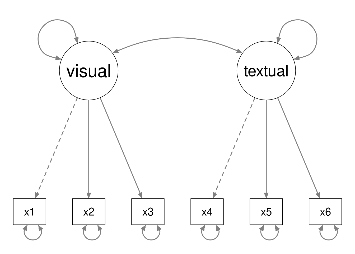
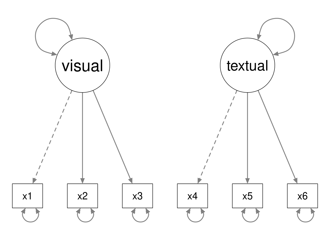
The second model is nested within the first model, because we can define the second model by fixing the latent covariance to zero in the first model.
Notice that the data contain \(6(6 + 1) / 2 = 21\) unique pieces of information. The first model estimates 13 parameters, and the second model estimates 12 parameters. Hence the first model has 8 degrees of freedom, and the second model has 9 degrees of freedom.
In general, the following must hold whenever Model B is nested within Model A.
- Model B will have fewer estimated parameters than Model A.
- Model B will have more degrees of freedom than Model A.
- Model A will be more complex than model B.
- Model A will fit the data better than model B.
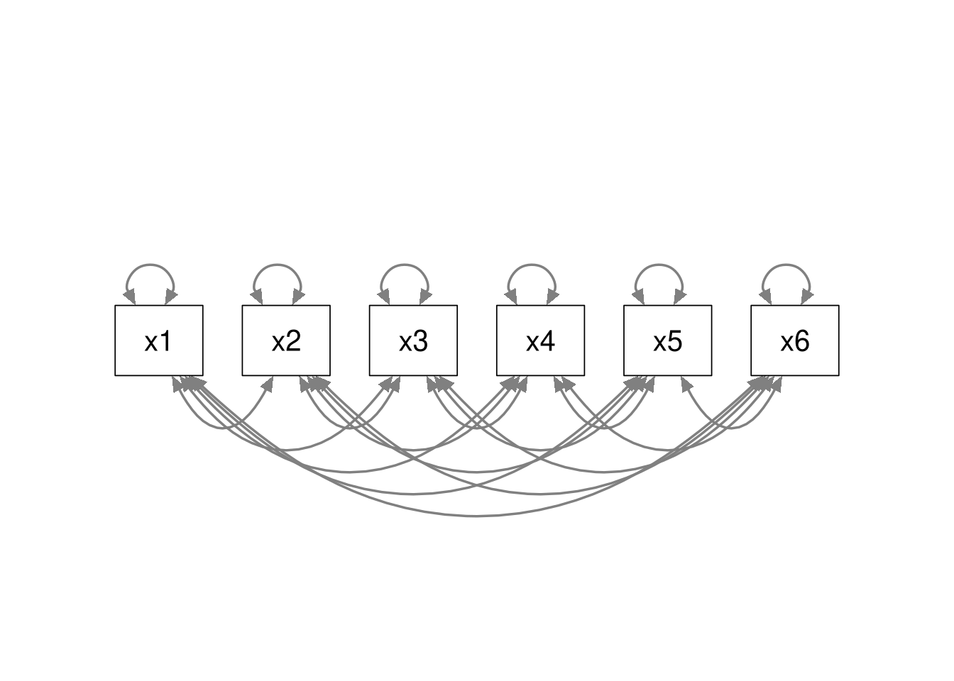
Saturated Model
All models are nested within the saturated model, because the saturated model estimates all possible relations among the variables. Regardless of what model we may be considering, we can always convert that model to a saturated model by estimating all possible associations. Hence, all models are nested within the saturated model.
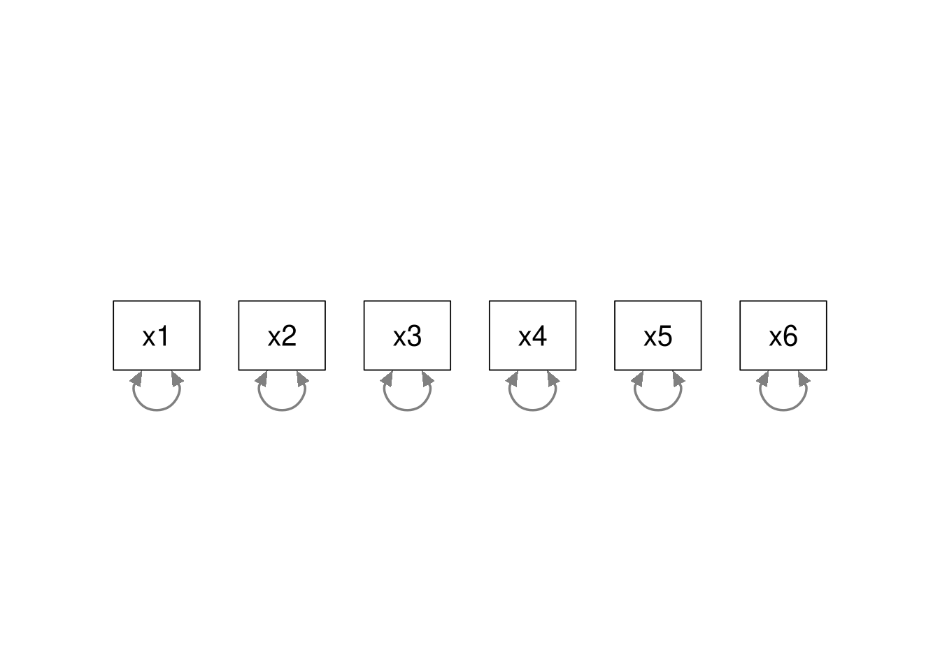
Baseline Model
Similarly, the baseline model (AKA, independence model) is nested within all other models. In the baseline model, we only estimate the variances of the observed items; all associations are constrained to zero. We can always convert our model to the baseline model by fixing all associations to zero. Hence, the baseline model is nested within all other models.
When two models are nested, we can use a \(\Delta \chi^2\) test to check if the nested model fits significantly worse than its parent model. Whenever we place constraints on the model, the fit will deteriorate, but we want to know if the constraints we imposed to define the nested model have produced too much loss of fit.
We can use the anova() function to easily conduct \(\Delta \chi^2\) tests comparing models that we’ve estimated with
cfa() or sem().
5.4.3.1
Use the anova() function to compare the three-factor model of Trust in Politics from 5.3.3 to the
one-factor model version 5.3.6.
- Explain what
Df,Chisq,Chisq diff,Df diff, andPr(>Chisq)mean. - Which model is more complex?
- Which model fits better?
- What is the conclusion of the test?
Click to show code
##
## Chi-Squared Difference Test
##
##        Df    AIC    BIC Chisq Chisq diff  RMSEA Df diff Pr(>Chisq)
## out_3f 62 742867 743088 10652
## out_1f 65 749876 750074 17667     7015.1 0.3977       3  < 2.2e-16
Click for explanation
Q1:
The Df column contains the degrees of freedom of each model.
- More df \(\Rightarrow\) Fewer estimated parameters \(\Rightarrow\) Less complex model
The Chisq column shows the \(\chi^2\) statistics (AKA, likelihood ratio statistics) for each model.
- Larger \(\chi^2\) \(\Rightarrow\) Worse fit
Chisq diff is the difference between the two \(\chi^2\) values (i.e., \(\Delta \chi^2\)).
- How much better the more complex model fits the data
- Larger \(\Delta \chi^2\) values indicate greater losses of fit induced by the constraints in the nested model.
Df diff is the difference in the degrees of freedom between the models.
- Since both models must be estimated from the same pool of variables, this difference also represents the number of parameters that were constrained to define the nested model.
Pr(>Chisq) is a p-value for the \(\Delta \chi^2\) test.
- \(H_0: \Delta \chi^2 = 0\)
- \(H_1: \Delta \chi^2 > 0\)
Q2:
The three-factor model has fewer degrees of freedom \((\textit{df} = 62)\) than the one-factor model \((\textit{df} = 65)\). So, the three-factor model is more complex.
Q3:
The three-factor model fits better than the one-factor model \((\chi_{3F}^2 = 10652.21\) vs. \(\chi_{1F}^2 = 17667.30)\).
Q4:
The three-factor model is more complex than the one-factor model, but the extra complexity is justified. The three-factor model fits significantly better than the one-factor model \((\Delta\chi^2 = 7015.1,\) \(\textit{df} = 3,\) \(p < 0.001).\)
5.4.3.2
Use the \(\Delta\chi^2\) to test if the additional parameter estimates you added in 5.4.2.2 and 5.4.2.4 significantly improve the model fit.
- Did the model fit significantly improve?
- Is the fit of the modified model acceptable?
Click to show code
##
## Chi-Squared Difference Test
##
##                 Df     AIC     BIC Chisq Chisq diff   RMSEA Df diff Pr(>Chisq)
## out_trust_att3 636 1422116 1422890 19151
## out_trust_att 638 1430291 1431050 27330 8179.2 0.59074 2 < 2.2e-16## npar fmin chisq
## 105.000 0.817 19150.640
## df pvalue baseline.chisq
## 636.000 0.000 201900.916
## baseline.df baseline.pvalue cfi
## 703.000 0.000 0.908
## tli nnfi rfi
## 0.898 0.898 0.895
## nfi pnfi ifi
## 0.905 0.819 0.908
## rni logl unrestricted.logl
## 0.908 -710953.076 -701377.756
## aic bic ntotal
## 1422116.153 1422889.867 11716.000
## bic2 rmsea rmsea.ci.lower
## 1422556.190 0.050 0.049
## rmsea.ci.upper rmsea.ci.level rmsea.pvalue
## 0.050 0.900 0.659
## rmsea.close.h0 rmsea.notclose.pvalue rmsea.notclose.h0
## 0.050 0.000 0.080
## rmr rmr_nomean srmr
## 0.152 0.152 0.045
## srmr_bentler srmr_bentler_nomean crmr
## 0.045 0.045 0.046
## crmr_nomean srmr_mplus srmr_mplus_nomean
## 0.046 0.045 0.045
## cn_05 cn_01 gfi
## 426.664 442.644 0.914
## agfi pgfi mfi
## 0.900 0.785 0.454
## ecvi
## 1.652Click for explanation
Yes, these modifications significantly improve the model fit \((\Delta\chi^2 = 8179.17,\) \(\textit{df} = 2,\) \(p < 0.001).\) In this case, the original 8-factor model is nested within the modified model. So, our \(\Delta \chi^2\) test is evaluating the improvement in fit contributed by freeing the two residual covariances. The \(\Delta \chi^2\) test is significant, so we can conclude that including the two new parameter estimates has significantly improved the model fit.
- I.e., Estimating these two residual covariances is “worth it” in the sense of balancing model fit and model complexity.
Also, the overall fit of the modified model is now more unambiguously acceptable \((\chi^2 = 19150.64,\) \(\textit{df} = 636,\) \(p < 0.001,\) \(\textrm{RMSEA} = 0.05,\) \(\textrm{CFI} = 0.908,\) \(\textrm{SRMR} = 0.045)\).
Very Important Caveat!
If we had found this result when testing our original model, we would be well-situated to proceed with our analysis. In this case, however, we are no longer justified in generalizing these estimates to the population. We only arrived at this well-fitting model by modifying our original theoretical model to better fit the data using estimates derived from those same data to guide our model modifications.
We’ve conducted this post-hoc analysis to help inform future research, and this result is useful as a starting point for future studies. Now, anyone analyzing these scales in the future could incorporate these residual covariances into their initial theoretical model. Basically, we conduct these types of post-hoc analyses to help future researchers learn from our mistakes.
5.4.3.3
Estimate a restricted version of the 8-factor CFA from 5.4.1.4.
- Remove all latent covariances between the three Trust in Politics factors and the five Attitudes Toward Immigration factors.
- Retain all other aspects of the original CFA.
Summarize the estimated model to check that everything worked.
Click to show code
First, we’ll define a syntax snippet to enforce the constraints.
constraints <- '
inst ~~ 0*immi + 0*social + 0*refugee + 0*cult + 0*econ
sat  ~~ 0*immi + 0*social + 0*refugee + 0*cult + 0*econ
pol  ~~ 0*immi + 0*social + 0*refugee + 0*cult + 0*econ
'
Now, we’ll add the constraint syntax to the CFA syntax.
Finally, we’ll estimate and summarize the restricted model.
out_trust_att0 <- cfa(mod_trust_att0, data = ess, std.lv = TRUE)
summary(out_trust_att0, fit.measures = TRUE, standardized = TRUE)
## lavaan 0.6-19 ended normally after 48 iterations
##
## Estimator ML
## Optimization method NLMINB
## Number of model parameters 89
## Number of equality constraints 1
##
## Used Total
## Number of observations 11716 19690
##
## Model Test User Model:
##
## Test statistic 29767.296
## Degrees of freedom 653
## P-value (Chi-square) 0.000
##
## Model Test Baseline Model:
##
## Test statistic 201900.916
## Degrees of freedom 703
## P-value 0.000
##
## User Model versus Baseline Model:
##
## Comparative Fit Index (CFI) 0.855
## Tucker-Lewis Index (TLI) 0.844
##
## Loglikelihood and Information Criteria:
##
## Loglikelihood user model (H0) -716261.405
## Loglikelihood unrestricted model (H1) -701377.756
##
## Akaike (AIC) 1432698.809
## Bayesian (BIC) 1433347.256
## Sample-size adjusted Bayesian (SABIC) 1433067.602
##
## Root Mean Square Error of Approximation:
##
## RMSEA 0.062
## 90 Percent confidence interval - lower 0.061
## 90 Percent confidence interval - upper 0.062
## P-value H_0: RMSEA <= 0.050 0.000
## P-value H_0: RMSEA >= 0.080 0.000
##
## Standardized Root Mean Square Residual:
##
## SRMR 0.099
##
## Parameter Estimates:
##
## Standard errors Standard
## Information Expected
## Information saturated (h1) model Structured
##
## Latent Variables:
## Estimate Std.Err z-value P(>|z|) Std.lv Std.all
## inst =~
## trstlgl 1.612 0.020 79.232 0.000 1.612 0.680
## trstplc 1.222 0.019 62.799 0.000 1.222 0.565
## trstun 1.471 0.020 73.119 0.000 1.471 0.639
## trstep 1.443 0.019 75.800 0.000 1.443 0.658
## trstprl 1.827 0.018 100.514 0.000 1.827 0.809
## sat =~
## stfhlth 1.170 0.021 56.653 0.000 1.170 0.526
## stfedu 1.305 0.020 64.284 0.000 1.305 0.585
## stfeco 1.652 0.020 82.421 0.000 1.652 0.712
## stfgov 1.716 0.019 88.703 0.000 1.716 0.752
## stfdem 1.604 0.019 85.172 0.000 1.604 0.730
## pol =~
## pltinvt 0.641 0.009 68.958 0.000 0.641 0.610
## pltcare 0.655 0.009 71.708 0.000 0.655 0.630
## trstplt 1.924 0.017 112.828 0.000 1.924 0.894
## immi =~
## imrcntr 0.608 0.007 92.827 0.000 0.608 0.744
## eimrcnt 0.576 0.007 84.288 0.000 0.576 0.693
## eimpcnt 0.694 0.006 125.076 0.000 0.694 0.903
## imsmetn 0.597 0.006 101.333 0.000 0.597 0.791
## impcntr 0.706 0.006 124.785 0.000 0.706 0.902
## imdfetn 0.695 0.006 121.763 0.000 0.695 0.889
## social =~
## imbgeco 1.561 0.018 85.019 0.000 1.561 0.720
## imbleco 1.296 0.019 69.034 0.000 1.296 0.613
## imwbcnt 1.640 0.017 95.993 0.000 1.640 0.786
## imwbcrm 1.120 0.018 62.069 0.000 1.120 0.562
## imtcjob 1.165 0.018 65.986 0.000 1.165 0.591
## imueclt 1.535 0.019 79.363 0.000 1.535 0.684
## refugee =~
## gvrfgap 0.673 0.009 71.904 0.000 0.673 0.647
## imrsprc 0.561 0.010 58.037 0.000 0.561 0.542
## rfgbfml 0.670 0.011 63.492 0.000 0.670 0.585
## rfggvfn 0.538 0.010 56.144 0.000 0.538 0.527
## rfgawrk 0.399 0.010 39.337 0.000 0.399 0.384
## rfgfrpc -0.544 0.009 -57.796 0.000 -0.544 -0.540
## shrrfg -0.664 0.009 -70.015 0.000 -0.664 -0.633
## cult =~
## qfimchr 1.839 0.029 64.271 0.000 1.839 0.632
## qfimwht 1.704 0.025 66.979 0.000 1.704 0.656
## pplstrd -0.663 0.011 -60.862 0.000 -0.663 -0.602
## vrtrlg 0.471 0.010 45.094 0.000 0.471 0.460
## econ =~
## imwgdwn (l) 0.754 0.008 98.038 0.000 0.754 0.706
## imhecop (l) 0.754 0.008 98.038 0.000 0.754 0.719
##
## Covariances:
## Estimate Std.Err z-value P(>|z|) Std.lv Std.all
## inst ~~
## immi 0.000 0.000 0.000
## social 0.000 0.000 0.000
## refugee 0.000 0.000 0.000
## cult 0.000 0.000 0.000
## econ 0.000 0.000 0.000
## sat ~~
## immi 0.000 0.000 0.000
## social 0.000 0.000 0.000
## refugee 0.000 0.000 0.000
## cult 0.000 0.000 0.000
## econ 0.000 0.000 0.000
## pol ~~
## immi 0.000 0.000 0.000
## social 0.000 0.000 0.000
## refugee 0.000 0.000 0.000
## cult 0.000 0.000 0.000
## econ 0.000 0.000 0.000
## inst ~~
## sat 0.747 0.006 117.182 0.000 0.747 0.747
## pol 0.877 0.005 180.127 0.000 0.877 0.877
## sat ~~
## pol 0.722 0.007 106.761 0.000 0.722 0.722
## immi ~~
## social -0.595 0.007 -82.989 0.000 -0.595 -0.595
## refugee 0.639 0.007 88.681 0.000 0.639 0.639
## cult 0.558 0.009 64.001 0.000 0.558 0.558
## econ -0.453 0.010 -45.844 0.000 -0.453 -0.453
## social ~~
## refugee -0.787 0.006 -128.158 0.000 -0.787 -0.787
## cult -0.540 0.010 -56.068 0.000 -0.540 -0.540
## econ 0.575 0.010 59.797 0.000 0.575 0.575
## refugee ~~
## cult 0.508 0.010 48.504 0.000 0.508 0.508
## econ -0.498 0.011 -45.912 0.000 -0.498 -0.498
## cult ~~
## econ -0.446 0.012 -37.300 0.000 -0.446 -0.446
##
## Variances:
## Estimate Std.Err z-value P(>|z|) Std.lv Std.all
## .trstlgl 3.014 0.045 66.962 0.000 3.014 0.537
## .trstplc 3.181 0.045 71.384 0.000 3.181 0.681
## .trstun 3.129 0.045 68.897 0.000 3.129 0.591
## .trstep 2.731 0.040 68.099 0.000 2.731 0.568
## .trstprl 1.763 0.032 54.918 0.000 1.763 0.346
## .stfhlth 3.573 0.050 71.120 0.000 3.573 0.723
## .stfedu 3.268 0.047 69.144 0.000 3.268 0.658
## .stfeco 2.653 0.043 61.756 0.000 2.653 0.493
## .stfgov 2.256 0.039 57.742 0.000 2.256 0.434
## .stfdem 2.254 0.037 60.124 0.000 2.254 0.467
## .pltinvt 0.692 0.010 69.925 0.000 0.692 0.627
## .pltcare 0.651 0.009 69.157 0.000 0.651 0.603
## .trstplt 0.931 0.031 30.402 0.000 0.931 0.201
## .imrcntr 0.298 0.004 70.928 0.000 0.298 0.446
## .eimrcnt 0.358 0.005 72.361 0.000 0.358 0.519
## .eimpcnt 0.109 0.002 56.138 0.000 0.109 0.185
## .imsmetn 0.213 0.003 68.962 0.000 0.213 0.375
## .impcntr 0.115 0.002 56.436 0.000 0.115 0.187
## .imdfetn 0.129 0.002 59.202 0.000 0.129 0.210
## .imbgeco 2.266 0.036 63.765 0.000 2.266 0.482
## .imbleco 2.792 0.040 69.449 0.000 2.792 0.624
## .imwbcnt 1.669 0.029 57.317 0.000 1.669 0.383
## .imwbcrm 2.720 0.038 71.120 0.000 2.720 0.684
## .imtcjob 2.532 0.036 70.225 0.000 2.532 0.651
## .imueclt 2.685 0.041 66.151 0.000 2.685 0.533
## .gvrfgap 0.628 0.010 64.853 0.000 0.628 0.581
## .imrsprc 0.756 0.011 69.846 0.000 0.756 0.706
## .rfgbfml 0.864 0.013 68.161 0.000 0.864 0.658
## .rfggvfn 0.752 0.011 70.363 0.000 0.752 0.722
## .rfgawrk 0.921 0.012 73.787 0.000 0.921 0.853
## .rfgfrpc 0.717 0.010 69.913 0.000 0.717 0.708
## .shrrfg 0.658 0.010 65.685 0.000 0.658 0.599
## .qfimchr 5.078 0.088 58.004 0.000 5.078 0.600
## .qfimwht 3.838 0.069 55.460 0.000 3.838 0.569
## .pplstrd 0.772 0.013 60.764 0.000 0.772 0.637
## .vrtrlg 0.825 0.012 69.206 0.000 0.825 0.788
## .imwgdwn 0.571 0.011 52.720 0.000 0.571 0.501
## .imhecop 0.531 0.010 50.693 0.000 0.531 0.483
## inst 1.000 1.000 1.000
## sat 1.000 1.000 1.000
## pol 1.000 1.000 1.000
## immi 1.000 1.000 1.000
## social 1.000 1.000 1.000
## refugee 1.000 1.000 1.000
## cult 1.000 1.000 1.000
## econ 1.000 1.000 1.000Below, you will conduct a \(\Delta\chi^2\) test to compare the full 8-factor CFA from 5.4.1.4 to the restricted version you estimated in 5.4.3.3. All remaining questions refer to this test.
5.4.3.4
- Which model is more complex?
- Which model has more degrees of freedom?
- What is the difference in the degrees of freedom between the models?
- How many degrees of freedom will we have for this test?
Click for explanation
- The unrestricted CFA is more complex: We estimate more parameters in that model.
- The restricted model will have more degrees of freedom: We lose one degree of freedom for every estimated parameter.
- \(\Delta \textit{df} = 24\): We fixed 24 latent covariances to define the restricted model, so the restricted model has 24 more degrees of freedom.
- Our \(\chi^2\) test will have \(\textit{df} = 24\): The df for a \(\Delta\chi^2\) is equal to the \(\Delta \textit{df}\) between the compared models.
5.4.3.5
Use R to conduct the \(\Delta\chi^2\) test.
- What is the conclusion of the test?
- Support your claim with appropriate statistics
Click to show code
##
## Chi-Squared Difference Test
##
##                 Df     AIC     BIC Chisq Chisq diff   RMSEA Df diff Pr(>Chisq)
## out_trust_att  638 1430291 1431050 27330
## out_trust_att0 653 1432699 1433347 29767     2437.5 0.11741      15  < 2.2e-16
Click for explanation
The unrestricted CFA fits significantly better than the restricted CFA \((\Delta\chi^2 = 2437.48,\) \(\textit{df} = 15,\) \(p < 0.001).\) Hence, the constraints imposed on the restricted model are untenable. The unrestricted CFA produces a significantly better representation of the data.
End of In-Class Exercises