4.4 In-Class Exercises
For this week’s in-class exercises, we’ll continue modeling the Cattell 16PF items using CFA. We will use the same dataset that you analyzed in the at-home exercises.
4.4.1
Load the cattell data.
- The relevant data are contained in the [canttell.rds][cattell_data] file.
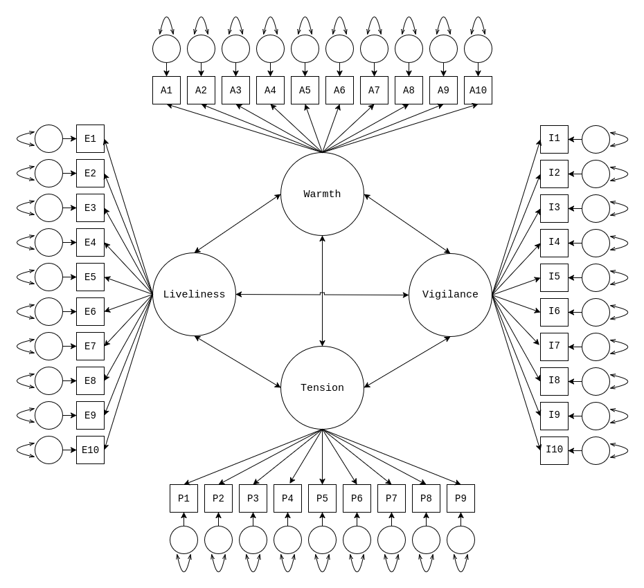
In the following exercises, we’ll work primarily with the four-factor CFA shown in the following path diagram. This CFA models the measurement of the Warmth, Liveliness, Vigilance, and Tension factors from the 16PF.
4.4.2
Calculate the following quantities for the CFA model shown above.
- The number of parameters in the model.
- The pieces of unique information provided by the data.
- The number of estimated parameters after applying the necessary scaling constraints.
- The degrees of freedom for the estimated model.
Click to show the answer
- The model contains 88 parameters
- 39 factor loadings
- 39 residual variances
- 4 latent variances
- 6 latent covariances
- Our model will include 39 observed variables, so the data provide 39 (39 + 1) / 2 = 780 pieces of information.
- To identify the covariance structure model, we need to fix one parameter in each factor’s sub-model. So, we will estimate 84 parameters.
- The estimated model will have 780 - 84 = 696 degrees of freedom.
4.4.3
Define the lavaan model syntax for the four-factor CFA shown above above.
- Do not specify any mean structure.
- Save this model syntax as an object in your environment.
Click to show code
4.4.4
Estimate the CFA model you defined in 4.4.3, and summarize the results.
- Use the
lavaan::cfa()function to estimate the model. - Use the “marker variable method” to set the scale of the latent factors.
- Use the default settings for the
cfa()function.
Click to show code
## Load the lavaan package:
library(lavaan)

## Estimate the CFA model:
outC1.1 <- cfa(mod1, data = cattell)

## Summarize the fitted model:
summary(outC1.1)
## lavaan 0.6-19 ended normally after 42 iterations
##
## Estimator ML
## Optimization method NLMINB
## Number of model parameters 84
##
## Number of observations 1000
##
## Model Test User Model:
##
## Test statistic 4238.359
## Degrees of freedom 696
## P-value (Chi-square) 0.000
##
## Parameter Estimates:
##
## Standard errors Standard
## Information Expected
## Information saturated (h1) model Structured
##
## Latent Variables:
## Estimate Std.Err z-value P(>|z|)
## warmth =~
## A1 1.000
## A2 0.962 0.050 19.056 0.000
## A3 0.772 0.053 14.567 0.000
## A4 0.790 0.050 15.654 0.000
## A5 0.927 0.050 18.449 0.000
## A6 0.847 0.049 17.261 0.000
## A7 0.792 0.049 16.257 0.000
## A8 -0.534 0.059 -9.127 0.000
## A9 -0.902 0.055 -16.552 0.000
## A10 -0.431 0.053 -8.068 0.000
## liveliness =~
## E1 1.000
## E2 1.273 0.055 23.226 0.000
## E3 0.488 0.042 11.713 0.000
## E4 1.166 0.052 22.405 0.000
## E5 0.342 0.035 9.696 0.000
## E6 0.783 0.050 15.667 0.000
## E7 -0.140 0.044 -3.172 0.002
## E8 -1.027 0.052 -19.799 0.000
## E9 -0.196 0.042 -4.642 0.000
## E10 -0.528 0.048 -10.944 0.000
## vigilance =~
## I1 1.000
## I2 1.252 0.092 13.589 0.000
## I3 0.915 0.079 11.629 0.000
## I4 1.585 0.105 15.059 0.000
## I5 0.769 0.077 9.997 0.000
## I6 1.153 0.089 12.972 0.000
## I7 -1.220 0.087 -13.986 0.000
## I8 -1.466 0.099 -14.748 0.000
## I9 -1.219 0.085 -14.295 0.000
## I10 -1.089 0.085 -12.835 0.000
## tension =~
## P1 1.000
## P2 0.908 0.035 25.697 0.000
## P3 0.577 0.036 15.960 0.000
## P4 0.582 0.035 16.780 0.000
## P5 0.361 0.031 11.730 0.000
## P6 0.449 0.036 12.619 0.000
## P7 0.425 0.038 11.271 0.000
## P8 -0.747 0.034 -21.836 0.000
## P9 -0.370 0.034 -10.964 0.000
##
## Covariances:
## Estimate Std.Err z-value P(>|z|)
## warmth ~~
## liveliness 0.245 0.025 9.690 0.000
## vigilance -0.207 0.021 -9.902 0.000
## tension -0.241 0.028 -8.641 0.000
## liveliness ~~
## vigilance -0.112 0.019 -6.000 0.000
## tension -0.030 0.031 -0.966 0.334
## vigilance ~~
## tension 0.305 0.029 10.440 0.000
##
## Variances:
## Estimate Std.Err z-value P(>|z|)
## .A1 0.594 0.030 19.593 0.000
## .A2 0.391 0.021 18.471 0.000
## .A3 0.711 0.034 20.991 0.000
## .A4 0.592 0.029 20.632 0.000
## .A5 0.427 0.022 19.052 0.000
## .A6 0.475 0.024 19.884 0.000
## .A7 0.521 0.026 20.388 0.000
## .A8 1.153 0.053 21.957 0.000
## .A9 0.634 0.031 20.254 0.000
## .A10 0.992 0.045 22.056 0.000
## .E1 0.693 0.037 18.840 0.000
## .E2 0.562 0.037 15.277 0.000
## .E3 0.890 0.041 21.722 0.000
## .E4 0.605 0.036 16.826 0.000
## .E5 0.681 0.031 21.950 0.000
## .E6 1.075 0.051 20.990 0.000
## .E7 1.194 0.053 22.321 0.000
## .E8 0.850 0.044 19.343 0.000
## .E9 1.076 0.048 22.275 0.000
## .E10 1.225 0.056 21.817 0.000
## .I1 0.981 0.046 21.501 0.000
## .I2 0.702 0.034 20.470 0.000
## .I3 0.818 0.038 21.498 0.000
## .I4 0.440 0.025 17.497 0.000
## .I5 0.991 0.045 21.858 0.000
## .I6 0.784 0.037 20.927 0.000
## .I7 0.546 0.027 20.046 0.000
## .I8 0.488 0.026 18.611 0.000
## .I9 0.457 0.023 19.598 0.000
## .I10 0.739 0.035 21.005 0.000
## .P1 0.392 0.029 13.380 0.000
## .P2 0.596 0.034 17.379 0.000
## .P3 0.958 0.045 21.160 0.000
## .P4 0.864 0.041 21.002 0.000
## .P5 0.758 0.035 21.769 0.000
## .P6 0.994 0.046 21.665 0.000
## .P7 1.145 0.052 21.819 0.000
## .P8 0.706 0.036 19.578 0.000
## .P9 0.919 0.042 21.850 0.000
## warmth 0.453 0.041 10.987 0.000
## liveliness 0.710 0.058 12.236 0.000
## vigilance 0.301 0.039 7.720 0.000
## tension 1.007 0.064 15.610 0.0004.4.5
Do the number of model parameters and degrees of freedom reported in the lavaan output agree with the values you calculated in 4.4.2?
Click to show answer
Yes, the values should agree. This first part of the lavaan model summary reports the number of model parameters and the degrees of freedom.
## lavaan 0.6-19 ended normally after 42 iterations
##
##   Estimator                                         ML
##   Optimization method                           NLMINB
##   Number of model parameters                        84
##
##   Number of observations                          1000
##
## Model Test User Model:
##
##   Test statistic                              4238.359
##   Degrees of freedom                               696
##   P-value (Chi-square)                           0.000
In this case, we see that we’ve estimated 84 parameters and we have df = 696.
4.4.6
Examine the factor loadings from the model you estimated in 4.4.4, and answer the following questions.
- Some of the estimated factor loadings are negative. Why are these particular loadings negative?
- Do you think the negative factor loadings are a problem? Explain you reasoning.
- Do the estimates make sense given the wording of the observed items and the putative meanings of the latent constructs?
Click to show answer
- The negative factor loadings are associated with reverse-coded items. Such items get negative factor loadings because higher scores on those items reflect lower levels of the latent construct. In other words, reverse coded items have negative item-scale correlations. \(\\[3pt]\)
- No, the negative factor loadings are not inherently problematic. Negative factor loadings do not have a deleterious
effect on the definition of the latent factor. That being said, negative factor loadings can complicate the analysis.
- Trying to set the scale by fixing the factor loading for a reverse coded item can cause estimation problems or flip the meaning of the latent factor.
- We need to be extra careful when placing constraints for hypothesis testing. \(\\[3pt]\)
- Yes, the estimated factor loadings largely align with theoretical expectations. For example, the observed items that appear to reflect interpersonal “warmth” are associated with positive factor loadings for the Warmth factor, and the reverse coded items that seem to indicate “coldness” have negative factor loadings. The same pattern holds for all four latent factors.
4.4.7
Interpret the latent covariances from the model you estimated in 4.4.4.
- Use the parameter estimates and statistical tests from your model to support your interpretations.
- Do the estimates make sense given the putative meanings of the latent constructs?
Click to show answer
The estimated latent covariances largely conform to theoretical expectations. The two “pro-social” factors, Warmth and Liveliness, are positively associated \((\psi_{2,1} = 0.245\), \(\textit{SE} = 0.025\), \(p < 0.001)\), as are the two “anti-social” factors, Vigilance and Tension, \((\psi_{4,3} = 0.305\), \(\textit{SE} = 0.029\), \(p < 0.001)\). Furthermore, Warmth negatively correlates with both of the “anti-social” factors (Vigilance: \(\psi_{3,1} = -0.207\), \(\textit{SE} = 0.021\), \(p < 0.001\); Tension: \(\psi_{4,1} = -0.241\), \(\textit{SE} = 0.028\), \(p < 0.001)\), and Liveliness negatively correlates with Vigilance \((\psi_{2,3} = -0.112\), \(\textit{SE} = 0.019\), \(p < 0.001)\). Only Liveliness and Tension are not significantly associated \((\psi_{2,4} = -0.03\), \(\textit{SE} = 0.031\), \(p = 0.334)\).
We can request more information when we summarize a fitted lavaan model by adding additional arguments to the
summary() call. For the purposes of this course, the following options are most useful.
ci = TRUE: Include confidence intervals for the estimated parametersstadardized = TRUE: Include the standardized parameter estimatesrsquare = TRUE: Include the \(R^2\) estimates for all endogenous variables in the modelfit.measures = TRUE: Include the model fit statisticsmodindices = TRUE: Include the modification indices
For example, the following code prints the summary including 95% confidence intervals for the parameter estimates.
## lavaan 0.6-19 ended normally after 42 iterations
##
##   Estimator                                         ML
##   Optimization method                           NLMINB
##   Number of model parameters                        84
##
##   Number of observations                          1000
##
## Model Test User Model:
##
##   Test statistic                              4238.359
##   Degrees of freedom                               696
##   P-value (Chi-square)                           0.000
##
## Parameter Estimates:
##
##   Standard errors                             Standard
##   Information                                 Expected
##   Information saturated (h1) model          Structured
##
## Latent Variables:
##                    Estimate  Std.Err  z-value  P(>|z|) ci.lower ci.upper
##   warmth =~
##     A1                1.000                               1.000    1.000
##     A2                0.962    0.050   19.056    0.000    0.863    1.060
##     A3                0.772    0.053   14.567    0.000    0.668    0.875
##     A4                0.790    0.050   15.654    0.000    0.691    0.889
##     A5                0.927    0.050   18.449    0.000    0.829    1.026
##     A6                0.847    0.049   17.261    0.000    0.750    0.943
##     A7                0.792    0.049   16.257    0.000    0.696    0.887
##     A8               -0.534    0.059   -9.127    0.000   -0.649   -0.419
##     A9               -0.902    0.055  -16.552    0.000   -1.009   -0.796
##     A10              -0.431    0.053   -8.068    0.000   -0.535   -0.326
##   liveliness =~
##     E1                1.000                               1.000    1.000
##     E2                1.273    0.055   23.226    0.000    1.166    1.380
##     E3                0.488    0.042   11.713    0.000    0.406    0.569
##     E4                1.166    0.052   22.405    0.000    1.064    1.267
##     E5                0.342    0.035    9.696    0.000    0.273    0.412
##     E6                0.783    0.050   15.667    0.000    0.685    0.881
##     E7               -0.140    0.044   -3.172    0.002   -0.227   -0.054
##     E8               -1.027    0.052  -19.799    0.000   -1.129   -0.926
##     E9               -0.196    0.042   -4.642    0.000   -0.279   -0.113
##     E10              -0.528    0.048  -10.944    0.000   -0.622   -0.433
##   vigilance =~
##     I1                1.000                               1.000    1.000
##     I2                1.252    0.092   13.589    0.000    1.072    1.433
##     I3                0.915    0.079   11.629    0.000    0.760    1.069
##     I4                1.585    0.105   15.059    0.000    1.378    1.791
##     I5                0.769    0.077    9.997    0.000    0.618    0.920
##     I6                1.153    0.089   12.972    0.000    0.979    1.328
##     I7               -1.220    0.087  -13.986    0.000   -1.392   -1.049
##     I8               -1.466    0.099  -14.748    0.000   -1.661   -1.271
##     I9               -1.219    0.085  -14.295    0.000   -1.387   -1.052
##     I10              -1.089    0.085  -12.835    0.000   -1.255   -0.923
##   tension =~
##     P1                1.000                               1.000    1.000
##     P2                0.908    0.035   25.697    0.000    0.838    0.977
##     P3                0.577    0.036   15.960    0.000    0.506    0.648
##     P4                0.582    0.035   16.780    0.000    0.514    0.650
##     P5                0.361    0.031   11.730    0.000    0.301    0.422
##     P6                0.449    0.036   12.619    0.000    0.379    0.518
##     P7                0.425    0.038   11.271    0.000    0.351    0.499
##     P8               -0.747    0.034  -21.836    0.000   -0.815   -0.680
##     P9               -0.370    0.034  -10.964    0.000   -0.436   -0.304
##
## Covariances:
##                    Estimate  Std.Err  z-value  P(>|z|) ci.lower ci.upper
##   warmth ~~
##     liveliness        0.245    0.025    9.690    0.000    0.196    0.295
##     vigilance        -0.207    0.021   -9.902    0.000   -0.248   -0.166
##     tension          -0.241    0.028   -8.641    0.000   -0.296   -0.187
##   liveliness ~~
##     vigilance        -0.112    0.019   -6.000    0.000   -0.149   -0.076
##     tension          -0.030    0.031   -0.966    0.334   -0.091    0.031
##   vigilance ~~
##     tension           0.305    0.029   10.440    0.000    0.248    0.362
##
## Variances:
##                    Estimate  Std.Err  z-value  P(>|z|) ci.lower ci.upper
##    .A1                0.594    0.030   19.593    0.000    0.534    0.653
##    .A2                0.391    0.021   18.471    0.000    0.350    0.433
##    .A3                0.711    0.034   20.991    0.000    0.645    0.778
##    .A4                0.592    0.029   20.632    0.000    0.536    0.648
##    .A5                0.427    0.022   19.052    0.000    0.383    0.471
##    .A6                0.475    0.024   19.884    0.000    0.428    0.522
##    .A7                0.521    0.026   20.388    0.000    0.471    0.571
##    .A8                1.153    0.053   21.957    0.000    1.050    1.256
##    .A9                0.634    0.031   20.254    0.000    0.573    0.695
##    .A10               0.992    0.045   22.056    0.000    0.904    1.080
##    .E1                0.693    0.037   18.840    0.000    0.621    0.765
##    .E2                0.562    0.037   15.277    0.000    0.490    0.634
##    .E3                0.890    0.041   21.722    0.000    0.809    0.970
##    .E4                0.605    0.036   16.826    0.000    0.535    0.676
##    .E5                0.681    0.031   21.950    0.000    0.620    0.742
##    .E6                1.075    0.051   20.990    0.000    0.975    1.176
##    .E7                1.194    0.053   22.321    0.000    1.089    1.299
##    .E8                0.850    0.044   19.343    0.000    0.764    0.936
##    .E9                1.076    0.048   22.275    0.000    0.981    1.171
##    .E10               1.225    0.056   21.817    0.000    1.115    1.335
##    .I1                0.981    0.046   21.501    0.000    0.892    1.070
##    .I2                0.702    0.034   20.470    0.000    0.635    0.770
##    .I3                0.818    0.038   21.498    0.000    0.743    0.893
##    .I4                0.440    0.025   17.497    0.000    0.391    0.489
##    .I5                0.991    0.045   21.858    0.000    0.902    1.080
##    .I6                0.784    0.037   20.927    0.000    0.711    0.858
##    .I7                0.546    0.027   20.046    0.000    0.492    0.599
##    .I8                0.488    0.026   18.611    0.000    0.437    0.539
##    .I9                0.457    0.023   19.598    0.000    0.411    0.503
##    .I10               0.739    0.035   21.005    0.000    0.670    0.808
##    .P1                0.392    0.029   13.380    0.000    0.335    0.450
##    .P2                0.596    0.034   17.379    0.000    0.529    0.664
##    .P3                0.958    0.045   21.160    0.000    0.869    1.047
##    .P4                0.864    0.041   21.002    0.000    0.784    0.945
##    .P5                0.758    0.035   21.769    0.000    0.690    0.827
##    .P6                0.994    0.046   21.665    0.000    0.904    1.084
##    .P7                1.145    0.052   21.819    0.000    1.042    1.248
##    .P8                0.706    0.036   19.578    0.000    0.635    0.777
##    .P9                0.919    0.042   21.850    0.000    0.836    1.001
##     warmth            0.453    0.041   10.987    0.000    0.372    0.534
##     liveliness        0.710    0.058   12.236    0.000    0.596    0.824
##     vigilance         0.301    0.039    7.720    0.000    0.224    0.377
##     tension           1.007    0.064   15.610    0.000    0.880    1.133
4.4.8
Summarize the model you estimated in 4.4.4, and include the standardized parameter estimates and the \(R^2\) values in the summary.
Click to show code
## lavaan 0.6-19 ended normally after 42 iterations
##
##   Estimator                                         ML
##   Optimization method                           NLMINB
##   Number of model parameters                        84
##
##   Number of observations                          1000
##
## Model Test User Model:
##
##   Test statistic                              4238.359
##   Degrees of freedom                               696
##   P-value (Chi-square)                           0.000
##
## Parameter Estimates:
##
##   Standard errors                             Standard
##   Information                                 Expected
##   Information saturated (h1) model          Structured
##
## Latent Variables:
##                    Estimate  Std.Err  z-value  P(>|z|)   Std.lv  Std.all
##   warmth =~
##     A1                1.000                               0.673    0.658
##     A2                0.962    0.050   19.056    0.000    0.647    0.719
##     A3                0.772    0.053   14.567    0.000    0.519    0.524
##     A4                0.790    0.050   15.654    0.000    0.532    0.569
##     A5                0.927    0.050   18.449    0.000    0.624    0.690
##     A6                0.847    0.049   17.261    0.000    0.570    0.637
##     A7                0.792    0.049   16.257    0.000    0.533    0.594
##     A8               -0.534    0.059   -9.127    0.000   -0.359   -0.317
##     A9               -0.902    0.055  -16.552    0.000   -0.607   -0.606
##     A10              -0.431    0.053   -8.068    0.000   -0.290   -0.279
##   liveliness =~
##     E1                1.000                               0.843    0.712
##     E2                1.273    0.055   23.226    0.000    1.073    0.820
##     E3                0.488    0.042   11.713    0.000    0.411    0.399
##     E4                1.166    0.052   22.405    0.000    0.982    0.784
##     E5                0.342    0.035    9.696    0.000    0.288    0.330
##     E6                0.783    0.050   15.667    0.000    0.660    0.537
##     E7               -0.140    0.044   -3.172    0.002   -0.118   -0.108
##     E8               -1.027    0.052  -19.799    0.000   -0.866   -0.685
##     E9               -0.196    0.042   -4.642    0.000   -0.165   -0.158
##     E10              -0.528    0.048  -10.944    0.000   -0.445   -0.373
##   vigilance =~
##     I1                1.000                               0.548    0.484
##     I2                1.252    0.092   13.589    0.000    0.687    0.634
##     I3                0.915    0.079   11.629    0.000    0.502    0.485
##     I4                1.585    0.105   15.059    0.000    0.869    0.795
##     I5                0.769    0.077    9.997    0.000    0.422    0.390
##     I6                1.153    0.089   12.972    0.000    0.633    0.581
##     I7               -1.220    0.087  -13.986    0.000   -0.669   -0.671
##     I8               -1.466    0.099  -14.748    0.000   -0.804   -0.755
##     I9               -1.219    0.085  -14.295    0.000   -0.669   -0.703
##     I10              -1.089    0.085  -12.835    0.000   -0.597   -0.570
##   tension =~
##     P1                1.000                               1.003    0.848
##     P2                0.908    0.035   25.697    0.000    0.911    0.763
##     P3                0.577    0.036   15.960    0.000    0.579    0.509
##     P4                0.582    0.035   16.780    0.000    0.584    0.532
##     P5                0.361    0.031   11.730    0.000    0.363    0.384
##     P6                0.449    0.036   12.619    0.000    0.450    0.411
##     P7                0.425    0.038   11.271    0.000    0.427    0.370
##     P8               -0.747    0.034  -21.836    0.000   -0.750   -0.666
##     P9               -0.370    0.034  -10.964    0.000   -0.371   -0.361
##
## Covariances:
##                    Estimate  Std.Err  z-value  P(>|z|)   Std.lv  Std.all
##   warmth ~~
##     liveliness        0.245    0.025    9.690    0.000    0.433    0.433
##     vigilance        -0.207    0.021   -9.902    0.000   -0.560   -0.560
##     tension          -0.241    0.028   -8.641    0.000   -0.358   -0.358
##   liveliness ~~
##     vigilance        -0.112    0.019   -6.000    0.000   -0.243   -0.243
##     tension          -0.030    0.031   -0.966    0.334   -0.035   -0.035
##   vigilance ~~
##     tension           0.305    0.029   10.440    0.000    0.554    0.554
##
## Variances:
##                    Estimate  Std.Err  z-value  P(>|z|)   Std.lv  Std.all
##    .A1                0.594    0.030   19.593    0.000    0.594    0.567
##    .A2                0.391    0.021   18.471    0.000    0.391    0.483
##    .A3                0.711    0.034   20.991    0.000    0.711    0.725
##    .A4                0.592    0.029   20.632    0.000    0.592    0.677
##    .A5                0.427    0.022   19.052    0.000    0.427    0.523
##    .A6                0.475    0.024   19.884    0.000    0.475    0.594
##    .A7                0.521    0.026   20.388    0.000    0.521    0.647
##    .A8                1.153    0.053   21.957    0.000    1.153    0.899
##    .A9                0.634    0.031   20.254    0.000    0.634    0.632
##    .A10               0.992    0.045   22.056    0.000    0.992    0.922
##    .E1                0.693    0.037   18.840    0.000    0.693    0.494
##    .E2                0.562    0.037   15.277    0.000    0.562    0.328
##    .E3                0.890    0.041   21.722    0.000    0.890    0.840
##    .E4                0.605    0.036   16.826    0.000    0.605    0.386
##    .E5                0.681    0.031   21.950    0.000    0.681    0.891
##    .E6                1.075    0.051   20.990    0.000    1.075    0.712
##    .E7                1.194    0.053   22.321    0.000    1.194    0.988
##    .E8                0.850    0.044   19.343    0.000    0.850    0.531
##    .E9                1.076    0.048   22.275    0.000    1.076    0.975
##    .E10               1.225    0.056   21.817    0.000    1.225    0.861
##    .I1                0.981    0.046   21.501    0.000    0.981    0.765
##    .I2                0.702    0.034   20.470    0.000    0.702    0.598
##    .I3                0.818    0.038   21.498    0.000    0.818    0.765
##    .I4                0.440    0.025   17.497    0.000    0.440    0.368
##    .I5                0.991    0.045   21.858    0.000    0.991    0.848
##    .I6                0.784    0.037   20.927    0.000    0.784    0.662
##    .I7                0.546    0.027   20.046    0.000    0.546    0.549
##    .I8                0.488    0.026   18.611    0.000    0.488    0.430
##    .I9                0.457    0.023   19.598    0.000    0.457    0.505
##    .I10               0.739    0.035   21.005    0.000    0.739    0.675
##    .P1                0.392    0.029   13.380    0.000    0.392    0.280
##    .P2                0.596    0.034   17.379    0.000    0.596    0.418
##    .P3                0.958    0.045   21.160    0.000    0.958    0.741
##    .P4                0.864    0.041   21.002    0.000    0.864    0.717
##    .P5                0.758    0.035   21.769    0.000    0.758    0.852
##    .P6                0.994    0.046   21.665    0.000    0.994    0.831
##    .P7                1.145    0.052   21.819    0.000    1.145    0.863
##    .P8                0.706    0.036   19.578    0.000    0.706    0.557
##    .P9                0.919    0.042   21.850    0.000    0.919    0.870
##     warmth            0.453    0.041   10.987    0.000    1.000    1.000
##     liveliness        0.710    0.058   12.236    0.000    1.000    1.000
##     vigilance         0.301    0.039    7.720    0.000    1.000    1.000
##     tension           1.007    0.064   15.610    0.000    1.000    1.000
##
## R-Square:
##                    Estimate
##     A1                0.433
##     A2                0.517
##     A3                0.275
##     A4                0.323
##     A5                0.477
##     A6                0.406
##     A7                0.353
##     A8                0.101
##     A9                0.368
##     A10               0.078
##     E1                0.506
##     E2                0.672
##     E3                0.160
##     E4                0.614
##     E5                0.109
##     E6                0.288
##     E7                0.012
##     E8                0.469
##     E9                0.025
##     E10               0.139
##     I1                0.235
##     I2                0.402
##     I3                0.235
##     I4                0.632
##     I5                0.152
##     I6                0.338
##     I7                0.451
##     I8                0.570
##     I9                0.495
##     I10               0.325
##     P1                0.720
##     P2                0.582
##     P3                0.259
##     P4                0.283
##     P5                0.148
##     P6                0.169
##     P7                0.137
##     P8                0.443
##     P9                0.130
We can extract specific elements from the fitted lavaan object with the lavInspect() function. For example, the
following code extracts the number of estimated parameters.
## [1] 844.4.9
Check the help file for the lavInspect() function to see what you can extract from a fitted lavaan object.
4.4.10
Use the lavInspect() function to extract the following data from the lavaan object you created in
4.4.4.
- The factor loading matrix
- The latent covariance matrix
- The estimated \(R^2\) values for the indicator variables.
Click to show code
# Extract the estimated parameter matrices
parEst <- lavInspect(outC1.1, "estimates")

# Print the estimated factor loading matrix
parEst$lambda
## warmth lvlnss viglnc tensin
## A1 1.000 0.000 0.000 0.000
## A2 0.962 0.000 0.000 0.000
## A3 0.772 0.000 0.000 0.000
## A4 0.790 0.000 0.000 0.000
## A5 0.927 0.000 0.000 0.000
## A6 0.847 0.000 0.000 0.000
## A7 0.792 0.000 0.000 0.000
## A8 -0.534 0.000 0.000 0.000
## A9 -0.902 0.000 0.000 0.000
## A10 -0.431 0.000 0.000 0.000
## E1 0.000 1.000 0.000 0.000
## E2 0.000 1.273 0.000 0.000
## E3 0.000 0.488 0.000 0.000
## E4 0.000 1.166 0.000 0.000
## E5 0.000 0.342 0.000 0.000
## E6 0.000 0.783 0.000 0.000
## E7 0.000 -0.140 0.000 0.000
## E8 0.000 -1.027 0.000 0.000
## E9 0.000 -0.196 0.000 0.000
## E10 0.000 -0.528 0.000 0.000
## I1 0.000 0.000 1.000 0.000
## I2 0.000 0.000 1.252 0.000
## I3 0.000 0.000 0.915 0.000
## I4 0.000 0.000 1.585 0.000
## I5 0.000 0.000 0.769 0.000
## I6 0.000 0.000 1.153 0.000
## I7 0.000 0.000 -1.220 0.000
## I8 0.000 0.000 -1.466 0.000
## I9 0.000 0.000 -1.219 0.000
## I10 0.000 0.000 -1.089 0.000
## P1 0.000 0.000 0.000 1.000
## P2 0.000 0.000 0.000 0.908
## P3 0.000 0.000 0.000 0.577
## P4 0.000 0.000 0.000 0.582
## P5 0.000 0.000 0.000 0.361
## P6 0.000 0.000 0.000 0.449
## P7 0.000 0.000 0.000 0.425
## P8 0.000 0.000 0.000 -0.747
## P9 0.000 0.000 0.000 -0.370## warmth lvlnss viglnc tensin
## warmth 0.453
## liveliness 0.245 0.710
## vigilance -0.207 -0.112 0.301
## tension -0.241 -0.030 0.305 1.007## warmth lvlnss viglnc tensin
## warmth 0.453
## liveliness 0.245 0.710
## vigilance -0.207 -0.112 0.301
## tension -0.241 -0.030 0.305 1.007## A1 A2 A3 A4 A5 A6 A7 A8 A9 A10 E1 E2 E3
## 0.433 0.517 0.275 0.323 0.477 0.406 0.353 0.101 0.368 0.078 0.506 0.672 0.160
## E4 E5 E6 E7 E8 E9 E10 I1 I2 I3 I4 I5 I6
## 0.614 0.109 0.288 0.012 0.469 0.025 0.139 0.235 0.402 0.235 0.632 0.152 0.338
## I7 I8 I9 I10 P1 P2 P3 P4 P5 P6 P7 P8 P9
## 0.451 0.570 0.495 0.325 0.720 0.582 0.259 0.283 0.148 0.169 0.137 0.443 0.1304.4.11
Re-specify the model from 4.4.4 by fixing all latent covariances to zero.
- Estimate the re-specified model.
- Summarize the fitted model object.
Click to show code
# Modify the lavaan model syntax to fix the latent covariances
mod1.2 <- '
warmth     =~ A1 + A2 + A3 + A4 + A5 + A6 + A7 + A8 + A9 + A10
liveliness =~ E1 + E2 + E3 + E4 + E5 + E6 + E7 + E8 + E9 + E10
vigilance  =~ I1 + I2 + I3 + I4 + I5 + I6 + I7 + I8 + I9 + I10
tension    =~ P1 + P2 + P3 + P4 + P5 + P6 + P7 + P8 + P9

liveliness ~~ 0*warmth
vigilance  ~~ 0*warmth + 0*liveliness
tension    ~~ 0*warmth + 0*liveliness + 0*vigilance
'

# Estimate the new model
outC1.2 <- cfa(mod1.2, data = cattell)
summary(outC1.2)
## lavaan 0.6-19 ended normally after 36 iterations
##
## Estimator ML
## Optimization method NLMINB
## Number of model parameters 78
##
## Number of observations 1000
##
## Model Test User Model:
##
## Test statistic 4930.129
## Degrees of freedom 702
## P-value (Chi-square) 0.000
##
## Parameter Estimates:
##
## Standard errors Standard
## Information Expected
## Information saturated (h1) model Structured
##
## Latent Variables:
## Estimate Std.Err z-value P(>|z|)
## warmth =~
## A1 1.000
## A2 0.908 0.049 18.670 0.000
## A3 0.796 0.052 15.342 0.000
## A4 0.786 0.049 15.952 0.000
## A5 0.893 0.049 18.362 0.000
## A6 0.831 0.048 17.422 0.000
## A7 0.783 0.047 16.505 0.000
## A8 -0.516 0.057 -8.996 0.000
## A9 -0.860 0.053 -16.269 0.000
## A10 -0.418 0.052 -7.979 0.000
## liveliness =~
## E1 1.000
## E2 1.285 0.056 23.041 0.000
## E3 0.476 0.042 11.330 0.000
## E4 1.177 0.053 22.271 0.000
## E5 0.325 0.036 9.128 0.000
## E6 0.792 0.051 15.672 0.000
## E7 -0.129 0.045 -2.887 0.004
## E8 -1.037 0.053 -19.730 0.000
## E9 -0.186 0.043 -4.365 0.000
## E10 -0.541 0.049 -11.115 0.000
## vigilance =~
## I1 1.000
## I2 1.308 0.101 12.946 0.000
## I3 0.939 0.085 11.082 0.000
## I4 1.669 0.117 14.257 0.000
## I5 0.789 0.082 9.586 0.000
## I6 1.188 0.096 12.312 0.000
## I7 -1.310 0.097 -13.454 0.000
## I8 -1.556 0.111 -14.036 0.000
## I9 -1.266 0.094 -13.527 0.000
## I10 -1.143 0.093 -12.313 0.000
## tension =~
## P1 1.000
## P2 0.903 0.035 26.164 0.000
## P3 0.545 0.036 15.343 0.000
## P4 0.551 0.034 16.163 0.000
## P5 0.353 0.030 11.701 0.000
## P6 0.434 0.035 12.446 0.000
## P7 0.403 0.037 10.890 0.000
## P8 -0.734 0.033 -21.961 0.000
## P9 -0.326 0.033 -9.826 0.000
##
## Covariances:
## Estimate Std.Err z-value P(>|z|)
## warmth ~~
## liveliness 0.000
## vigilance 0.000
## liveliness ~~
## vigilance 0.000
## warmth ~~
## tension 0.000
## liveliness ~~
## tension 0.000
## vigilance ~~
## tension 0.000
##
## Variances:
## Estimate Std.Err z-value P(>|z|)
## .A1 0.571 0.030 18.989 0.000
## .A2 0.419 0.023 18.565 0.000
## .A3 0.680 0.033 20.572 0.000
## .A4 0.582 0.029 20.325 0.000
## .A5 0.438 0.023 18.847 0.000
## .A6 0.472 0.024 19.548 0.000
## .A7 0.513 0.026 20.067 0.000
## .A8 1.156 0.053 21.921 0.000
## .A9 0.652 0.032 20.182 0.000
## .A10 0.993 0.045 22.025 0.000
## .E1 0.700 0.037 18.824 0.000
## .E2 0.553 0.037 14.893 0.000
## .E3 0.899 0.041 21.752 0.000
## .E4 0.597 0.036 16.530 0.000
## .E5 0.690 0.031 21.992 0.000
## .E6 1.070 0.051 20.934 0.000
## .E7 1.197 0.054 22.327 0.000
## .E8 0.843 0.044 19.214 0.000
## .E9 1.079 0.048 22.283 0.000
## .E10 1.217 0.056 21.779 0.000
## .I1 1.008 0.047 21.535 0.000
## .I2 0.705 0.035 20.333 0.000
## .I3 0.828 0.039 21.474 0.000
## .I4 0.432 0.026 16.914 0.000
## .I5 0.998 0.046 21.842 0.000
## .I6 0.798 0.038 20.884 0.000
## .I7 0.523 0.027 19.608 0.000
## .I8 0.471 0.026 18.021 0.000
## .I9 0.465 0.024 19.470 0.000
## .I10 0.738 0.035 20.884 0.000
## .P1 0.352 0.030 11.786 0.000
## .P2 0.571 0.034 16.758 0.000
## .P3 0.982 0.046 21.266 0.000
## .P4 0.887 0.042 21.119 0.000
## .P5 0.759 0.035 21.771 0.000
## .P6 1.000 0.046 21.685 0.000
## .P7 1.157 0.053 21.857 0.000
## .P8 0.704 0.036 19.509 0.000
## .P9 0.945 0.043 21.957 0.000
## warmth 0.475 0.042 11.229 0.000
## liveliness 0.703 0.058 12.125 0.000
## vigilance 0.274 0.038 7.289 0.000
## tension 1.047 0.066 15.950 0.000Alternatively, we can keep the original model string and tell the cfa() function not to estimate any latent
covariances by setting the option orthogonal.x = TRUE.
## lavaan 0.6-19 ended normally after 36 iterations
##
##   Estimator                                         ML
##   Optimization method                           NLMINB
##   Number of model parameters                        78
##
##   Number of observations                          1000
##
## Model Test User Model:
##
##   Test statistic                              4930.129
##   Degrees of freedom                               702
##   P-value (Chi-square)                           0.000
##
## Parameter Estimates:
##
##   Standard errors                             Standard
##   Information                                 Expected
##   Information saturated (h1) model          Structured
##
## Latent Variables:
##                    Estimate  Std.Err  z-value  P(>|z|)
##   warmth =~
##     A1                1.000
##     A2                0.908    0.049   18.670    0.000
##     A3                0.796    0.052   15.342    0.000
##     A4                0.786    0.049   15.952    0.000
##     A5                0.893    0.049   18.362    0.000
##     A6                0.831    0.048   17.422    0.000
##     A7                0.783    0.047   16.505    0.000
##     A8               -0.516    0.057   -8.996    0.000
##     A9               -0.860    0.053  -16.269    0.000
##     A10              -0.418    0.052   -7.979    0.000
##   liveliness =~
##     E1                1.000
##     E2                1.285    0.056   23.041    0.000
##     E3                0.476    0.042   11.330    0.000
##     E4                1.177    0.053   22.271    0.000
##     E5                0.325    0.036    9.128    0.000
##     E6                0.792    0.051   15.672    0.000
##     E7               -0.129    0.045   -2.887    0.004
##     E8               -1.037    0.053  -19.730    0.000
##     E9               -0.186    0.043   -4.365    0.000
##     E10              -0.541    0.049  -11.115    0.000
##   vigilance =~
##     I1                1.000
##     I2                1.308    0.101   12.946    0.000
##     I3                0.939    0.085   11.082    0.000
##     I4                1.669    0.117   14.257    0.000
##     I5                0.789    0.082    9.586    0.000
##     I6                1.188    0.096   12.312    0.000
##     I7               -1.310    0.097  -13.454    0.000
##     I8               -1.556    0.111  -14.036    0.000
##     I9               -1.266    0.094  -13.527    0.000
##     I10              -1.143    0.093  -12.313    0.000
##   tension =~
##     P1                1.000
##     P2                0.903    0.035   26.164    0.000
##     P3                0.545    0.036   15.343    0.000
##     P4                0.551    0.034   16.163    0.000
##     P5                0.353    0.030   11.701    0.000
##     P6                0.434    0.035   12.446    0.000
##     P7                0.403    0.037   10.890    0.000
##     P8               -0.734    0.033  -21.961    0.000
##     P9               -0.326    0.033   -9.826    0.000
##
## Covariances:
##                    Estimate  Std.Err  z-value  P(>|z|)
##   warmth ~~
##     liveliness        0.000
##     vigilance         0.000
##     tension           0.000
##   liveliness ~~
##     vigilance         0.000
##     tension           0.000
##   vigilance ~~
##     tension           0.000
##
## Variances:
##                    Estimate  Std.Err  z-value  P(>|z|)
##    .A1                0.571    0.030   18.989    0.000
##    .A2                0.419    0.023   18.565    0.000
##    .A3                0.680    0.033   20.572    0.000
##    .A4                0.582    0.029   20.325    0.000
##    .A5                0.438    0.023   18.847    0.000
##    .A6                0.472    0.024   19.548    0.000
##    .A7                0.513    0.026   20.067    0.000
##    .A8                1.156    0.053   21.921    0.000
##    .A9                0.652    0.032   20.182    0.000
##    .A10               0.993    0.045   22.025    0.000
##    .E1                0.700    0.037   18.824    0.000
##    .E2                0.553    0.037   14.893    0.000
##    .E3                0.899    0.041   21.752    0.000
##    .E4                0.597    0.036   16.530    0.000
##    .E5                0.690    0.031   21.992    0.000
##    .E6                1.070    0.051   20.934    0.000
##    .E7                1.197    0.054   22.327    0.000
##    .E8                0.843    0.044   19.214    0.000
##    .E9                1.079    0.048   22.283    0.000
##    .E10               1.217    0.056   21.779    0.000
##    .I1                1.008    0.047   21.535    0.000
##    .I2                0.705    0.035   20.333    0.000
##    .I3                0.828    0.039   21.474    0.000
##    .I4                0.432    0.026   16.914    0.000
##    .I5                0.998    0.046   21.842    0.000
##    .I6                0.798    0.038   20.884    0.000
##    .I7                0.523    0.027   19.608    0.000
##    .I8                0.471    0.026   18.021    0.000
##    .I9                0.465    0.024   19.470    0.000
##    .I10               0.738    0.035   20.884    0.000
##    .P1                0.352    0.030   11.786    0.000
##    .P2                0.571    0.034   16.758    0.000
##    .P3                0.982    0.046   21.266    0.000
##    .P4                0.887    0.042   21.119    0.000
##    .P5                0.759    0.035   21.771    0.000
##    .P6                1.000    0.046   21.685    0.000
##    .P7                1.157    0.053   21.857    0.000
##    .P8                0.704    0.036   19.509    0.000
##    .P9                0.945    0.043   21.957    0.000
##     warmth            0.475    0.042   11.229    0.000
##     liveliness        0.703    0.058   12.125    0.000
##     vigilance         0.274    0.038    7.289    0.000
##     tension           1.047    0.066   15.950    0.000
4.4.12
Compare the factor loadings for the Warmth construct from the following two models:
Are the factor loading matrices equal or different across models? What’s going on here? How would you explain the differences (or lack thereof)?
Click to show code
# Factor loadings from the correlated-factor CFA
lavInspect(outC1.1, "estimates")$lambda[1:10, 1, drop = FALSE]
## warmth
## A1 1.0000000
## A2 0.9615773
## A3 0.7715174
## A4 0.7904305
## A5 0.9271921
## A6 0.8465595
## A7 0.7915340
## A8 -0.5341244
## A9 -0.9023822
## A10 -0.4305772# Factor loadings from the orthogonal-factor CFA
lavInspect(outC1.2, "estimates")$lambda[1:10, 1, drop = FALSE]## warmth
## A1 1.0000000
## A2 0.9076620
## A3 0.7961509
## A4 0.7855184
## A5 0.8931789
## A6 0.8305816
## A7 0.7828006
## A8 -0.5159300
## A9 -0.8597832
## A10 -0.4177278Click for explanation
The models produce slightly different factor loadings because the different latent covariance structures imply subtly different definitions of the Warmth factor.
- M1 is the more flexible and “accurate” of the two models.
- The latent covariance structure of the CFA is fully saturated. So, the estimator has the best possible chance of fitting the data well (more details on what we mean by “fitting the data” coming next week).
- M2 imposes very strong constraints on the model structure.
- The model forces independence between the latent constructs. So, M2 “tries” to estimate a Warmth factor that best conforms to a reality wherein Warmth, Liveliness, Vigilance, and Tension are completely unrelated concepts.
M1 is the more appropriate way of estimating these four latent factors. M2 places untenable constraints on the latent covariance structure. These Draconian constraints influence the estimates of other model parameters in ways that we probably don’t want (unless we have good reason to force an orthogonal definition of these constructs).
End of In-Class Exercises