7.3 At-Home Exercises
This week, we’ll take another look at the Kestilä (2006) results. During this practical, you will use SEM to conduct a regression analysis of the Trust in Politics factors that you estimated in the Week 5 At-Home Exercises.
7.3.1
Load the Finnish subsample of ESS data.
- The relevant data are contained in the ess_finland.rds file.
- This dataset comprises the Finnish subsample from the Week 5 exercise data.
- The missing values have been imputed with a single round of predictive mean matching.
Note: Unless otherwise noted, all the following analyses use these data.
We need to do a little data processing before we can fit the regression model. At the moment, lavaan will not
automatically convert a factor variable into dummy codes. So, we need to create explicit dummy codes for the two factors
we’ll use as predictors in our regression analysis: sex and political orientation.
7.3.2
Convert the sex and political interest factors into dummy codes.
Click to show code
library(dplyr)

## Create a dummy codes by broadcasting a logical test on the factor levels:
ess_fin <- mutate(ess_fin,
                  female = ifelse(sex == "Female", 1, 0),
                  hi_pol_interest = ifelse(polintr_bin == "High Interest", 1, 0)
                  )

## Check the results:
with(ess_fin, table(dummy = female, factor = sex))
## factor
## dummy Male Female
## 0 960 0
## 1 0 1040## factor
## dummy Low Interest High Interest
## 0 1070 0
## 1 0 930Click for explanation
In R, we have several ways of converting a factor into an appropriate set of dummy codes.
- We could use the
dplyr::recode()function. - We can use the
model.matrix()function to define a design matrix based on the inherent contrast attribute of the factor.- Missing data will cause problems here.
- We can us
as.numeric()to revert the factor to its underlying numeric representation {Male = 1, Female = 2} and use arithmetic to convert {1, 2} \(\rightarrow\) {0, 1}.
When our factor only has two levels, though, the ifelse() function is the simplest way.
We are now ready to estimate our latent regression model. Specifically, we want to estimate a single SEM to regress the three Trust in Politics factors onto the following predictors:
- Sex
- Age
- Years of Education
- High vs. Low Political Interest
- Placement on the Left-Right Political Scale
The following path diagram shows the intended theoretical model.
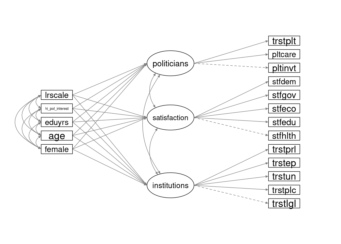
Although the variances are not included in this path diagram, all variables in the model (including the observed predictor variables) are random.
7.3.3
Define the lavaan model syntax for the SEM shown above.
- Use the definition of the
institutions,satsifaction, andpoliticiansfactors from 5.3.2 to define the DVs. - Covary the three latent factors.
- Covary the five predictors.
Click to show code
mod_sem <- '
## Define the latent DVs:
institutions =~ trstlgl + trstplc + trstun + trstep + trstprl
satisfaction =~ stfhlth + stfedu  + stfeco + stfgov + stfdem
politicians  =~ pltinvt + pltcare + trstplt

## Specify the structural relations:
institutions ~ female + age + eduyrs + hi_pol_interest + lrscale
satisfaction ~ female + age + eduyrs + hi_pol_interest + lrscale
politicians  ~ female + age + eduyrs + hi_pol_interest + lrscale
'
Click for explanation
We simply need to add a three lines defining the latent regression paths to our old CFA syntax.
We don’t need to specify the covariances in the syntax. We can use options in the
sem()function to request those estimates.
7.3.4
Estimate the SEM, and summarize the results.
- Fit the model to the processed Finnish subsample from above.
- Estimate the model using
lavaan::sem(). - Use the fixed-factor method to identify the model.
- Request the standardized parameter estimates with the summary.
- Request the \(R^2\) estimates with the summary.
Click to show code
library(lavaan)

## Fit the SEM:
out_sem <- sem(mod_sem, data = ess_fin, std.lv = TRUE, fixed.x = FALSE)

## Summarize the results:
summary(out_sem, fit.measures = TRUE, standardized = TRUE, rsquare = TRUE)
## lavaan 0.6-19 ended normally after 55 iterations
##
## Estimator ML
## Optimization method NLMINB
## Number of model parameters 59
##
## Number of observations 2000
##
## Model Test User Model:
##
## Test statistic 1496.911
## Degrees of freedom 112
## P-value (Chi-square) 0.000
##
## Model Test Baseline Model:
##
## Test statistic 12585.801
## Degrees of freedom 143
## P-value 0.000
##
## User Model versus Baseline Model:
##
## Comparative Fit Index (CFI) 0.889
## Tucker-Lewis Index (TLI) 0.858
##
## Loglikelihood and Information Criteria:
##
## Loglikelihood user model (H0) -67186.539
## Loglikelihood unrestricted model (H1) -66438.083
##
## Akaike (AIC) 134491.078
## Bayesian (BIC) 134821.531
## Sample-size adjusted Bayesian (SABIC) 134634.085
##
## Root Mean Square Error of Approximation:
##
## RMSEA 0.079
## 90 Percent confidence interval - lower 0.075
## 90 Percent confidence interval - upper 0.082
## P-value H_0: RMSEA <= 0.050 0.000
## P-value H_0: RMSEA >= 0.080 0.267
##
## Standardized Root Mean Square Residual:
##
## SRMR 0.045
##
## Parameter Estimates:
##
## Standard errors Standard
## Information Expected
## Information saturated (h1) model Structured
##
## Latent Variables:
## Estimate Std.Err z-value P(>|z|) Std.lv Std.all
## institutions =~
## trstlgl 1.421 0.043 32.812 0.000 1.473 0.676
## trstplc 0.886 0.037 23.972 0.000 0.918 0.523
## trstun 1.255 0.042 29.956 0.000 1.301 0.629
## trstep 1.609 0.042 38.286 0.000 1.668 0.758
## trstprl 1.727 0.039 43.722 0.000 1.790 0.832
## satisfaction =~
## stfhlth 0.965 0.043 22.428 0.000 0.999 0.499
## stfedu 0.637 0.032 20.082 0.000 0.659 0.452
## stfeco 1.251 0.038 32.805 0.000 1.294 0.682
## stfgov 1.606 0.036 44.697 0.000 1.662 0.854
## stfdem 1.501 0.036 41.212 0.000 1.553 0.806
## politicians =~
## pltinvt 0.557 0.021 26.903 0.000 0.588 0.579
## pltcare 0.543 0.019 28.427 0.000 0.573 0.606
## trstplt 1.813 0.039 46.980 0.000 1.916 0.908
##
## Regressions:
## Estimate Std.Err z-value P(>|z|) Std.lv Std.all
## institutions ~
## female 0.023 0.049 0.464 0.642 0.022 0.011
## age -0.006 0.001 -3.765 0.000 -0.005 -0.099
## eduyrs 0.025 0.007 3.595 0.000 0.025 0.096
## hi_pol_interst 0.275 0.051 5.360 0.000 0.265 0.132
## lrscale 0.077 0.012 6.262 0.000 0.074 0.150
## satisfaction ~
## female -0.111 0.049 -2.254 0.024 -0.107 -0.053
## age -0.007 0.001 -4.997 0.000 -0.007 -0.131
## eduyrs 0.000 0.007 0.065 0.948 0.000 0.002
## hi_pol_interst 0.168 0.051 3.313 0.001 0.163 0.081
## lrscale 0.104 0.012 8.465 0.000 0.101 0.203
## politicians ~
## female 0.047 0.049 0.949 0.342 0.044 0.022
## age -0.009 0.001 -5.797 0.000 -0.008 -0.150
## eduyrs 0.014 0.007 1.993 0.046 0.013 0.052
## hi_pol_interst 0.512 0.052 9.854 0.000 0.485 0.242
## lrscale 0.070 0.012 5.736 0.000 0.067 0.135
##
## Covariances:
## Estimate Std.Err z-value P(>|z|) Std.lv Std.all
## .institutions ~~
## .satisfaction 0.794 0.013 60.535 0.000 0.794 0.794
## .politicians 0.911 0.011 81.926 0.000 0.911 0.911
## .satisfaction ~~
## .politicians 0.705 0.016 42.897 0.000 0.705 0.705
## female ~~
## age 0.281 0.207 1.361 0.174 0.281 0.030
## eduyrs 0.121 0.044 2.782 0.005 0.121 0.062
## hi_pol_interst -0.019 0.006 -3.453 0.001 -0.019 -0.077
## lrscale -0.023 0.023 -0.997 0.319 -0.023 -0.022
## age ~~
## eduyrs -27.303 1.724 -15.833 0.000 -27.303 -0.379
## hi_pol_interst 1.151 0.208 5.539 0.000 1.151 0.125
## lrscale 1.707 0.837 2.040 0.041 1.707 0.046
## eduyrs ~~
## hi_pol_interst 0.318 0.044 7.207 0.000 0.318 0.163
## lrscale 0.827 0.177 4.665 0.000 0.827 0.105
## hi_pol_interest ~~
## lrscale 0.027 0.023 1.212 0.225 0.027 0.027
##
## Variances:
## Estimate Std.Err z-value P(>|z|) Std.lv Std.all
## .trstlgl 2.584 0.090 28.711 0.000 2.584 0.543
## .trstplc 2.242 0.074 30.339 0.000 2.242 0.727
## .trstun 2.584 0.088 29.367 0.000 2.584 0.604
## .trstep 2.062 0.077 26.863 0.000 2.062 0.426
## .trstprl 1.430 0.061 23.428 0.000 1.430 0.308
## .stfhlth 3.011 0.100 30.187 0.000 3.011 0.751
## .stfedu 1.689 0.055 30.510 0.000 1.689 0.795
## .stfeco 1.925 0.069 27.788 0.000 1.925 0.535
## .stfgov 1.028 0.053 19.519 0.000 1.028 0.271
## .stfdem 1.297 0.056 23.151 0.000 1.297 0.350
## .pltinvt 0.685 0.023 29.682 0.000 0.685 0.664
## .pltcare 0.566 0.019 29.373 0.000 0.566 0.632
## .trstplt 0.781 0.067 11.572 0.000 0.781 0.175
## .institutions 1.000 0.930 0.930
## .satisfaction 1.000 0.934 0.934
## .politicians 1.000 0.896 0.896
## female 0.250 0.008 31.623 0.000 0.250 1.000
## age 341.765 10.808 31.623 0.000 341.765 1.000
## eduyrs 15.221 0.481 31.623 0.000 15.221 1.000
## hi_pol_interst 0.249 0.008 31.623 0.000 0.249 1.000
## lrscale 4.089 0.129 31.623 0.000 4.089 1.000
##
## R-Square:
## Estimate
## trstlgl 0.457
## trstplc 0.273
## trstun 0.396
## trstep 0.574
## trstprl 0.692
## stfhlth 0.249
## stfedu 0.205
## stfeco 0.465
## stfgov 0.729
## stfdem 0.650
## pltinvt 0.336
## pltcare 0.368
## trstplt 0.825
## institutions 0.070
## satisfaction 0.066
## politicians 0.104Click for explanation
The fixed.x = FALSE argument tells lavaan to model the predictors as random variables. By default, lavaan will
covary any random predictor variables. So, we don’t need to make any other changes to the usual procedure.
In the final part of these exercises, you will rerun the above SEM as a path model wherein the observed mean scores
representing Trust in Institutions, Satisfaction with Political Systems, and Trust in Politicians act as the DVs.
The scoreItems() function from the psych package makes it very easy to create scale scores.
7.3.5
Read the documentation for the psych::scoreItems() function.
7.3.6
Use the psych::scoreItems() function to create mean scores to represent the three latent constructs in the above SEM.
Click to show code
library(psych)

## Create a list to define the item-to-score mapping
scaleKeys <- list(
  ins_score = c("trstlgl", "trstplc", "trstun", "trstep", "trstprl"),
  sat_score = c("stfhlth", "stfedu", "stfeco", "stfgov", "stfdem"),
  pol_score  = c("pltinvt", "pltcare", "trstplt")
  )

## Create the scale scores
scaleScores <- scoreItems(keys = scaleKeys, items = ess_fin, impute = "none")

## If we print the 'scaleScores' object, we get a bunch of interesting psychometric information
scaleScores
## Call: scoreItems(keys = scaleKeys, items = ess_fin, impute = "none")
##
## (Standardized) Alpha:
## ins_score sat_score pol_score
## alpha 0.82 0.8 0.69
##
## Standard errors of unstandardized Alpha:
## ins_score sat_score pol_score
## ASE 0.013 0.014 0.023
##
## Standardized Alpha of observed scales:
## ins_score sat_score pol_score
## [1,] 0.82 0.8 0.69
##
## Average item correlation:
## ins_score sat_score pol_score
## average.r 0.48 0.44 0.42
##
## Median item correlation:
## ins_score sat_score pol_score
## 0.48 0.38 0.53
##
## Guttman 6* reliability:
## ins_score sat_score pol_score
## Lambda.6 0.83 0.79 0.78
##
## Signal/Noise based upon av.r :
## ins_score sat_score pol_score
## Signal/Noise 4.7 3.9 2.2
##
## Scale intercorrelations corrected for attenuation
## raw correlations below the diagonal, alpha on the diagonal
## corrected correlations above the diagonal:
##
## Note that these are the correlations of the complete scales based on the correlation matrix,
## not the observed scales based on the raw items.
## ins_score sat_score pol_score
## ins_score 0.82 0.79 0.93
## sat_score 0.64 0.80 0.74
## pol_score 0.70 0.55 0.69
##
## Average adjusted correlations within and between scales (MIMS)
## ins_s st_sc pl_sc
## ins_score 0.48
## sat_score 1.41 0.44
## pol_score 1.28 0.87 0.42
##
## Average adjusted item x scale correlations within and between scales (MIMT)
## ins_s st_sc pl_sc
## ins_score 0.77
## sat_score 0.47 0.74
## pol_score 0.53 0.42 0.82
##
## In order to see the item by scale loadings and frequency counts of the data
## print with the short option = FALSE7.3.7
Use the mean scores you created above to estimate a path analytic version of the SEM from 7.3.4.
Click to show code
## Specify the model syntax for the path model:
mod_pa <- '
## Specify the structural relations:
ins_score ~ female + age + eduyrs + hi_pol_interest + lrscale
sat_score ~ female + age + eduyrs + hi_pol_interest + lrscale
pol_score ~ female + age + eduyrs + hi_pol_interest + lrscale
'

## Fit the path analytic model:
out_pa <- sem(mod_pa, data = ess_fin, fixed.x = FALSE)

## Summarize the results:
summary(out_pa, fit.measures = TRUE, standardized = TRUE, rsquare = TRUE)
## lavaan 0.6-19 ended normally after 45 iterations
##
## Estimator ML
## Optimization method NLMINB
## Number of model parameters 36
##
## Number of observations 2000
##
## Model Test User Model:
##
## Test statistic 0.000
## Degrees of freedom 0
##
## Model Test Baseline Model:
##
## Test statistic 2812.483
## Degrees of freedom 18
## P-value 0.000
##
## User Model versus Baseline Model:
##
## Comparative Fit Index (CFI) 1.000
## Tucker-Lewis Index (TLI) 1.000
##
## Loglikelihood and Information Criteria:
##
## Loglikelihood user model (H0) -30059.623
## Loglikelihood unrestricted model (H1) -30059.623
##
## Akaike (AIC) 60191.246
## Bayesian (BIC) 60392.879
## Sample-size adjusted Bayesian (SABIC) 60278.505
##
## Root Mean Square Error of Approximation:
##
## RMSEA 0.000
## 90 Percent confidence interval - lower 0.000
## 90 Percent confidence interval - upper 0.000
## P-value H_0: RMSEA <= 0.050 NA
## P-value H_0: RMSEA >= 0.080 NA
##
## Standardized Root Mean Square Residual:
##
## SRMR 0.000
##
## Parameter Estimates:
##
## Standard errors Standard
## Information Expected
## Information saturated (h1) model Structured
##
## Regressions:
## Estimate Std.Err z-value P(>|z|) Std.lv Std.all
## ins_score ~
## female 0.050 0.070 0.715 0.475 0.050 0.016
## age -0.007 0.002 -3.334 0.001 -0.007 -0.081
## eduyrs 0.034 0.010 3.434 0.001 0.034 0.084
## hi_pol_interst 0.332 0.072 4.588 0.000 0.332 0.104
## lrscale 0.106 0.017 6.133 0.000 0.106 0.135
## sat_score ~
## female -0.136 0.061 -2.248 0.025 -0.136 -0.049
## age -0.010 0.002 -5.350 0.000 -0.010 -0.129
## eduyrs -0.008 0.009 -0.936 0.349 -0.008 -0.023
## hi_pol_interst 0.160 0.062 2.560 0.010 0.160 0.058
## lrscale 0.135 0.015 9.031 0.000 0.135 0.198
## pol_score ~
## female 0.045 0.049 0.915 0.360 0.045 0.020
## age -0.010 0.001 -6.889 0.000 -0.010 -0.162
## eduyrs 0.020 0.007 2.878 0.004 0.020 0.069
## hi_pol_interst 0.541 0.050 10.722 0.000 0.541 0.236
## lrscale 0.064 0.012 5.270 0.000 0.064 0.113
##
## Covariances:
## Estimate Std.Err z-value P(>|z|) Std.lv Std.all
## .ins_score ~~
## .sat_score 1.317 0.055 23.934 0.000 1.317 0.634
## .pol_score 1.152 0.046 25.303 0.000 1.152 0.686
## .sat_score ~~
## .pol_score 0.782 0.037 21.263 0.000 0.782 0.540
## female ~~
## age 0.281 0.207 1.361 0.174 0.281 0.030
## eduyrs 0.122 0.044 2.782 0.005 0.122 0.062
## hi_pol_interst -0.019 0.006 -3.453 0.001 -0.019 -0.077
## lrscale -0.023 0.023 -0.997 0.319 -0.023 -0.022
## age ~~
## eduyrs -27.303 1.724 -15.833 0.000 -27.303 -0.379
## hi_pol_interst 1.151 0.208 5.539 0.000 1.151 0.125
## lrscale 1.707 0.837 2.040 0.041 1.707 0.046
## eduyrs ~~
## hi_pol_interst 0.318 0.044 7.207 0.000 0.318 0.163
## lrscale 0.827 0.177 4.665 0.000 0.827 0.105
## hi_pol_interest ~~
## lrscale 0.027 0.023 1.212 0.225 0.027 0.027
##
## Variances:
## Estimate Std.Err z-value P(>|z|) Std.lv Std.all
## .ins_score 2.410 0.076 31.623 0.000 2.410 0.949
## .sat_score 1.792 0.057 31.623 0.000 1.792 0.943
## .pol_score 1.169 0.037 31.623 0.000 1.169 0.895
## female 0.250 0.008 31.623 0.000 0.250 1.000
## age 341.765 10.808 31.623 0.000 341.765 1.000
## eduyrs 15.222 0.481 31.623 0.000 15.222 1.000
## hi_pol_interst 0.249 0.008 31.623 0.000 0.249 1.000
## lrscale 4.089 0.129 31.623 0.000 4.089 1.000
##
## R-Square:
## Estimate
## ins_score 0.051
## sat_score 0.057
## pol_score 0.1057.3.8
Compare the results from the path analysis to the SEM-based results.
- Does it matter whether we use a latent variable or a factor score to define the DV?
Hint: When comparing parameter estimates, use the fully standardized estimates (i.e., the values in the column labeled
Std.all).
Click to show code
Note: The “supportFunction.R” script that we source below isn’t a necessary part of the solution. This script defines
a bunch of convenience functions. One of these functions, partSummary(), allows us to print selected pieces of the
model summary.
## Source the script that defines the partSummary() convenience function:
source(here::here("code", "supportFunctions.R"))
## Regressions:
## Estimate Std.Err z-value P(>|z|) Std.lv Std.all
## institutions ~
## female 0.023 0.049 0.464 0.642 0.022 0.011
## age -0.006 0.001 -3.765 0.000 -0.005 -0.099
## eduyrs 0.025 0.007 3.595 0.000 0.025 0.096
## hi_pol_interst 0.275 0.051 5.360 0.000 0.265 0.132
## lrscale 0.077 0.012 6.262 0.000 0.074 0.150
## satisfaction ~
## female -0.111 0.049 -2.254 0.024 -0.107 -0.053
## age -0.007 0.001 -4.997 0.000 -0.007 -0.131
## eduyrs 0.000 0.007 0.065 0.948 0.000 0.002
## hi_pol_interst 0.168 0.051 3.313 0.001 0.163 0.081
## lrscale 0.104 0.012 8.465 0.000 0.101 0.203
## politicians ~
## female 0.047 0.049 0.949 0.342 0.044 0.022
## age -0.009 0.001 -5.797 0.000 -0.008 -0.150
## eduyrs 0.014 0.007 1.993 0.046 0.013 0.052
## hi_pol_interst 0.512 0.052 9.854 0.000 0.485 0.242
## lrscale 0.070 0.012 5.736 0.000 0.067 0.135## View the regression estimates from the path analysis:
partSummary(out_pa, 7, standardized = TRUE)## Regressions:
## Estimate Std.Err z-value P(>|z|) Std.lv Std.all
## ins_score ~
## female 0.050 0.070 0.715 0.475 0.050 0.016
## age -0.007 0.002 -3.334 0.001 -0.007 -0.081
## eduyrs 0.034 0.010 3.434 0.001 0.034 0.084
## hi_pol_interst 0.332 0.072 4.588 0.000 0.332 0.104
## lrscale 0.106 0.017 6.133 0.000 0.106 0.135
## sat_score ~
## female -0.136 0.061 -2.248 0.025 -0.136 -0.049
## age -0.010 0.002 -5.350 0.000 -0.010 -0.129
## eduyrs -0.008 0.009 -0.936 0.349 -0.008 -0.023
## hi_pol_interst 0.160 0.062 2.560 0.010 0.160 0.058
## lrscale 0.135 0.015 9.031 0.000 0.135 0.198
## pol_score ~
## female 0.045 0.049 0.915 0.360 0.045 0.020
## age -0.010 0.001 -6.889 0.000 -0.010 -0.162
## eduyrs 0.020 0.007 2.878 0.004 0.020 0.069
## hi_pol_interst 0.541 0.050 10.722 0.000 0.541 0.236
## lrscale 0.064 0.012 5.270 0.000 0.064 0.113## R-Square:
## Estimate
## trstlgl 0.457
## trstplc 0.273
## trstun 0.396
## trstep 0.574
## trstprl 0.692
## stfhlth 0.249
## stfedu 0.205
## stfeco 0.465
## stfgov 0.729
## stfdem 0.650
## pltinvt 0.336
## pltcare 0.368
## trstplt 0.825
## institutions 0.070
## satisfaction 0.066
## politicians 0.104## R-Square:
## Estimate
## ins_score 0.051
## sat_score 0.057
## pol_score 0.105Click for explanation
The two approaches reach the same substantive conclusions, but we do see differences. For example, the standardized regression weights mostly suggests larger effect sizes in the SEM model.
DV = Institutions
| X | SEM | PA |
|---|---|---|
| female | 0.011 | 0.016 |
| age | -0.099 | -0.081 |
| eduyrs | 0.096 | 0.084 |
| hi_pol_interest | 0.132 | 0.104 |
| lrscale | 0.150 | 0.135 |
DV = Satisfaction
| X | SEM | PA |
|---|---|---|
| female | -0.053 | -0.049 |
| age | -0.131 | -0.129 |
| eduyrs | 0.002 | -0.023 |
| hi_pol_interest | 0.081 | 0.058 |
| lrscale | 0.203 | 0.198 |
DV = Politicians
| X | SEM | PA |
|---|---|---|
| female | 0.022 | 0.020 |
| age | -0.150 | -0.162 |
| eduyrs | 0.052 | 0.069 |
| hi_pol_interest | 0.242 | 0.236 |
| lrscale | 0.135 | 0.113 |
The \(R^2\) values from the SEM are also larger than those from the path analysis for two out of three factors and approximately equal for the Politicians factor.
| SEM | PA | |
|---|---|---|
| institutions | 0.070 | 0.051 |
| satisfaction | 0.066 | 0.057 |
| politicians | 0.104 | 0.105 |
End of At-Home Exercises