4.3 At-Home Exercises
This week, we will take our first steps into the world of factor analysis. We’ll begin by fitting some CFA models using personality scale data.
4.3.1 Setup
Data:
You will use the following dataset for these exercises.
This dataset contains 1000 observations of 16X personality items collected as part of the International Personality Item Pool. These items are meant to assess Raymond Cattell’s 16 personality factors (16PF):
- Warmth
- Reasoning
- Emotional Stability
- Dominance
- Liveliness
- Rule-Consciousness
- Social Boldness
- Sensitivity
- Vigilance
- Abstractness
- Privateness
- Apprehension
- Openness to Change
- Self-Reliance
- Perfectionism
- Tension
The 16PF Wikipedia page provides a nice summary of the scale.
Packages:
To complete these exercises, you will need to install the package described below.
| Package | Description |
|---|---|
| semPlot | Programmatically draw path diagrams in R |
Use the install.packages() function to install this package.
4.3.2
Load the cattell data.
- The relevant data are contained in the [canttell.rds][cattell_data] file.
We’ll first estimate a simple one-dimensional CFA of the Warmth factor. Our target model is defined as follows:
- One reflective latent factor representing the Warmth dimension
- 10 observed indicators: {
A1,A2, …,A10} - 10 residual variances but no residual covariances
Basically, our CFA should estimate the default measurement model through which one latent factor generates 10 observed indicator variables.
4.3.3
Sketch a path diagram of the CFA model described above.
- Use pencil and paper (or the equivalent); don’t generate the diagram programmatically.
4.3.4
Calculate the following quantities for the Warmth CFA described above.
- The number of parameters in the model.
- The pieces of unique information provided by the data.
- The number of estimated parameters after applying the necessary scaling constraints.
- The degrees of freedom for the estimated model.
Click to show the answer
- The model contains 21 parameters
- 10 factor loadings
- 10 residual variances
- One latent variance
- Our model will include 10 observed variables, so the data provide 10 (10 + 1) / 2 = 55 pieces of information.
- To identify the covariance structure model, we need to fix one parameter. So, we will estimate 20 parameters.
- The estimated model will have 55 - 20 = 35 degrees of freedom.
4.3.5
Define the lavaan model syntax for the unidimensional CFA of Warmth described above.
- Do not specify any mean structure.
- Save this model syntax as an object in your environment.
Click to show code
Click for explanation
At this point, we only need to define the factor loading map. We can specify all the other options when we estimate the model.
4.3.6
Estimate the CFA model you defined in 4.3.5, and summarize the results.
- Use the
lavaan::cfa()function to estimate the model. - Use the default settings for the
cfa()function.
Check the results, and answer the following questions:
- What is the estimated variance of the Warmth factor?
- How is the model identified when using the default settings?
Click to show code
## Load the lavaan package:
library(lavaan)

## Estimate the CFA model:
outH1.1 <- cfa(mod1, data = cattell)

## Summarize the fitted model:
summary(outH1.1)
## lavaan 0.6-19 ended normally after 23 iterations
##
## Estimator ML
## Optimization method NLMINB
## Number of model parameters 20
##
## Number of observations 1000
##
## Model Test User Model:
##
## Test statistic 336.181
## Degrees of freedom 35
## P-value (Chi-square) 0.000
##
## Parameter Estimates:
##
## Standard errors Standard
## Information Expected
## Information saturated (h1) model Structured
##
## Latent Variables:
## Estimate Std.Err z-value P(>|z|)
## warmth =~
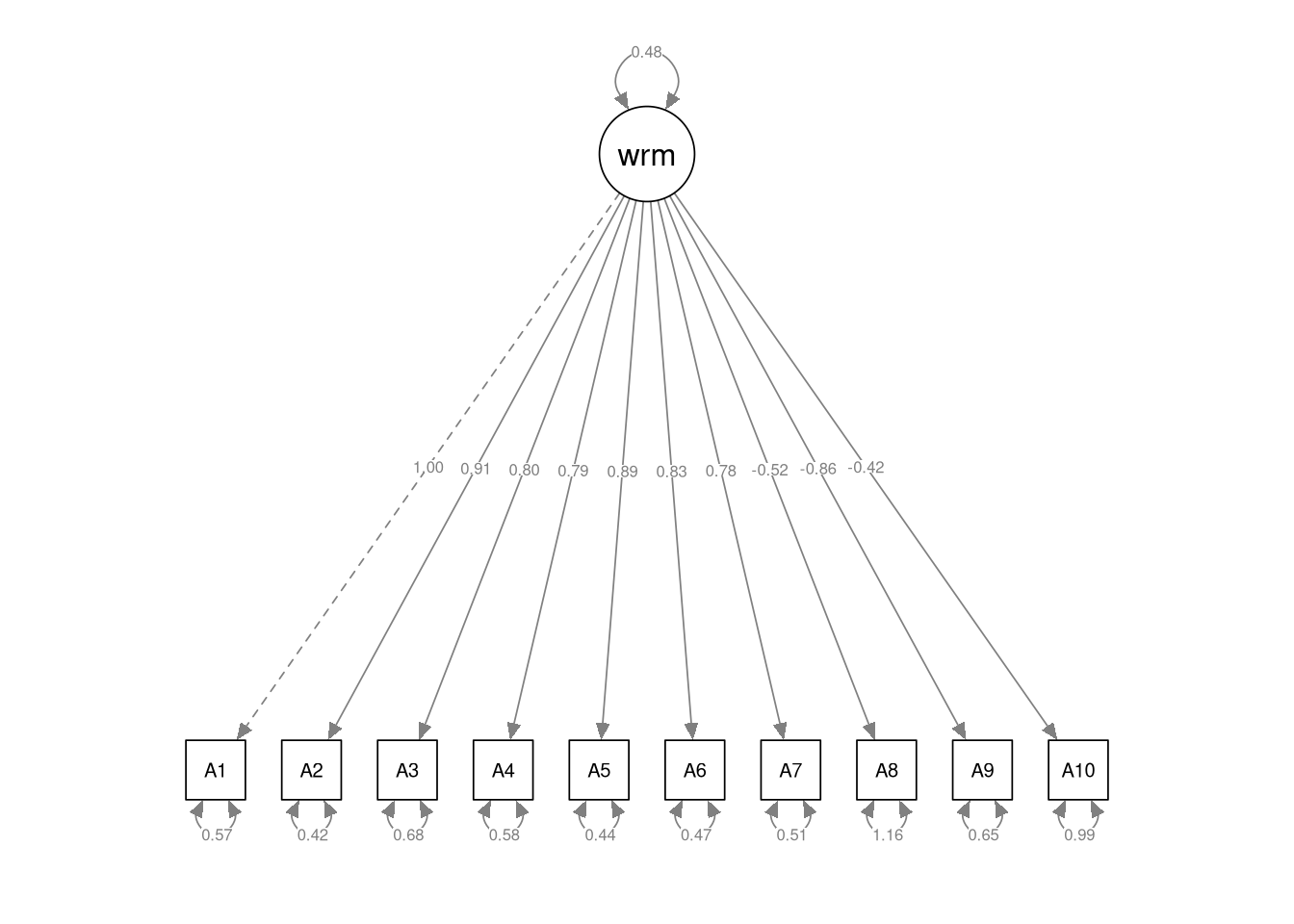
## A1 1.000
## A2 0.908 0.049 18.670 0.000
## A3 0.796 0.052 15.342 0.000
## A4 0.786 0.049 15.952 0.000
## A5 0.893 0.049 18.362 0.000
## A6 0.831 0.048 17.422 0.000
## A7 0.783 0.047 16.505 0.000
## A8 -0.516 0.057 -8.996 0.000
## A9 -0.860 0.053 -16.269 0.000
## A10 -0.418 0.052 -7.979 0.000
##
## Variances:
## Estimate Std.Err z-value P(>|z|)
## .A1 0.571 0.030 18.989 0.000
## .A2 0.419 0.023 18.565 0.000
## .A3 0.680 0.033 20.572 0.000
## .A4 0.582 0.029 20.325 0.000
## .A5 0.438 0.023 18.847 0.000
## .A6 0.472 0.024 19.548 0.000
## .A7 0.513 0.026 20.067 0.000
## .A8 1.156 0.053 21.921 0.000
## .A9 0.652 0.032 20.182 0.000
## .A10 0.993 0.045 22.025 0.000
## warmth 0.475 0.042 11.229 0.000Click for explanation
The estimated latent variance is \(\psi_{11} = 0.475\).
The cfa() function is just a wrapper for the lavaan() function with several options set at the defaults you would
want for a standard CFA.
- By default, the model is identified by fixing the first factor loading of each factor to 1 (due to the argument
auto.fix.first = TRUE).
To see a full list of the (many) options you can specify to tweak the behavior of lavaan estimation functions run
?lavOptions.
4.3.7
Do the number of model parameters and degrees of freedom reported in the lavaan output agree with the values you calculated in 4.3.4?
Click to show answer
Yes, the values should agree. This first part of the lavaan model summary reports the number of model parameters and the degrees of freedom.
## lavaan 0.6-19 ended normally after 23 iterations
##
##   Estimator                                         ML
##   Optimization method                           NLMINB
##   Number of model parameters                        20
##
##   Number of observations                          1000
##
## Model Test User Model:
##
##   Test statistic                               336.181
##   Degrees of freedom                                35
##   P-value (Chi-square)                           0.000
In this case, we see that we’ve estimated 20 parameters and we have df = 35.
4.3.8
Use the semPaths() function from the semPlot package to draw a path diagram of your estimated CFA.
- Include the parameter estimates in the diagram.
Now, we’re going to complicate matters slightly by adding another dimension to our model. We’ll now estimate a two-dimensional CFA that contains correlated Warmth and Dominance factors.
Defined this new model as follows:
- Two correlated, reflective latent factors: one Warmth factor and one Dominance factor
- 10 observed indicators of Warmth: {
A1,A2, …,A10} - 10 observed indicators of Dominance: {
D1,D2, …,D10} - No cross-loadings
- No residual correlations
Again, this CFA should estimate the default measurement model though which two correlated latent factors generate a set of 20 observed indicators.
4.3.9
Sketch a path diagram of the CFA model described above.
- Use pencil and paper (or the equivalent); don’t generate the diagram programmatically.
4.3.10
Define the lavaan model syntax for a two-factor model of the Warmth and Dominance items.
- Save this syntax as an object in your environment.
Click to show code
4.3.11
Estimate the two-factor model you specified in 4.3.10, and summarize the results.
- Identify the model by fixing the first factor loading of each construct to 1.
- Do not estimate any mean structure.
Click to show code
## Estimate the two factor model:
outH2.1 <- cfa(mod2, data = cattell)

## Summarize the results:
summary(outH2.1)
## lavaan 0.6-19 ended normally after 26 iterations
##
## Estimator ML
## Optimization method NLMINB
## Number of model parameters 41
##
## Number of observations 1000
##
## Model Test User Model:
##
## Test statistic 1158.738
## Degrees of freedom 169
## P-value (Chi-square) 0.000
##
## Parameter Estimates:
##
## Standard errors Standard
## Information Expected
## Information saturated (h1) model Structured
##
## Latent Variables:
## Estimate Std.Err z-value P(>|z|)
## warmth =~
## A1 1.000
## A2 0.908 0.048 18.880 0.000
## A3 0.780 0.051 15.188 0.000
## A4 0.771 0.049 15.829 0.000
## A5 0.900 0.048 18.679 0.000
## A6 0.835 0.047 17.684 0.000
## A7 0.773 0.047 16.468 0.000
## A8 -0.508 0.057 -8.921 0.000
## A9 -0.847 0.052 -16.199 0.000
## A10 -0.414 0.052 -7.954 0.000
## dominance =~
## D1 1.000
## D2 0.774 0.040 19.507 0.000
## D3 0.500 0.041 12.244 0.000
## D4 0.462 0.042 11.078 0.000
## D5 0.841 0.034 24.730 0.000
## D6 0.449 0.034 13.166 0.000
## D7 -0.875 0.040 -22.044 0.000
## D8 -0.426 0.036 -11.774 0.000
## D9 -0.712 0.039 -18.223 0.000
## D10 -0.630 0.046 -13.799 0.000
##
## Covariances:
## Estimate Std.Err z-value P(>|z|)
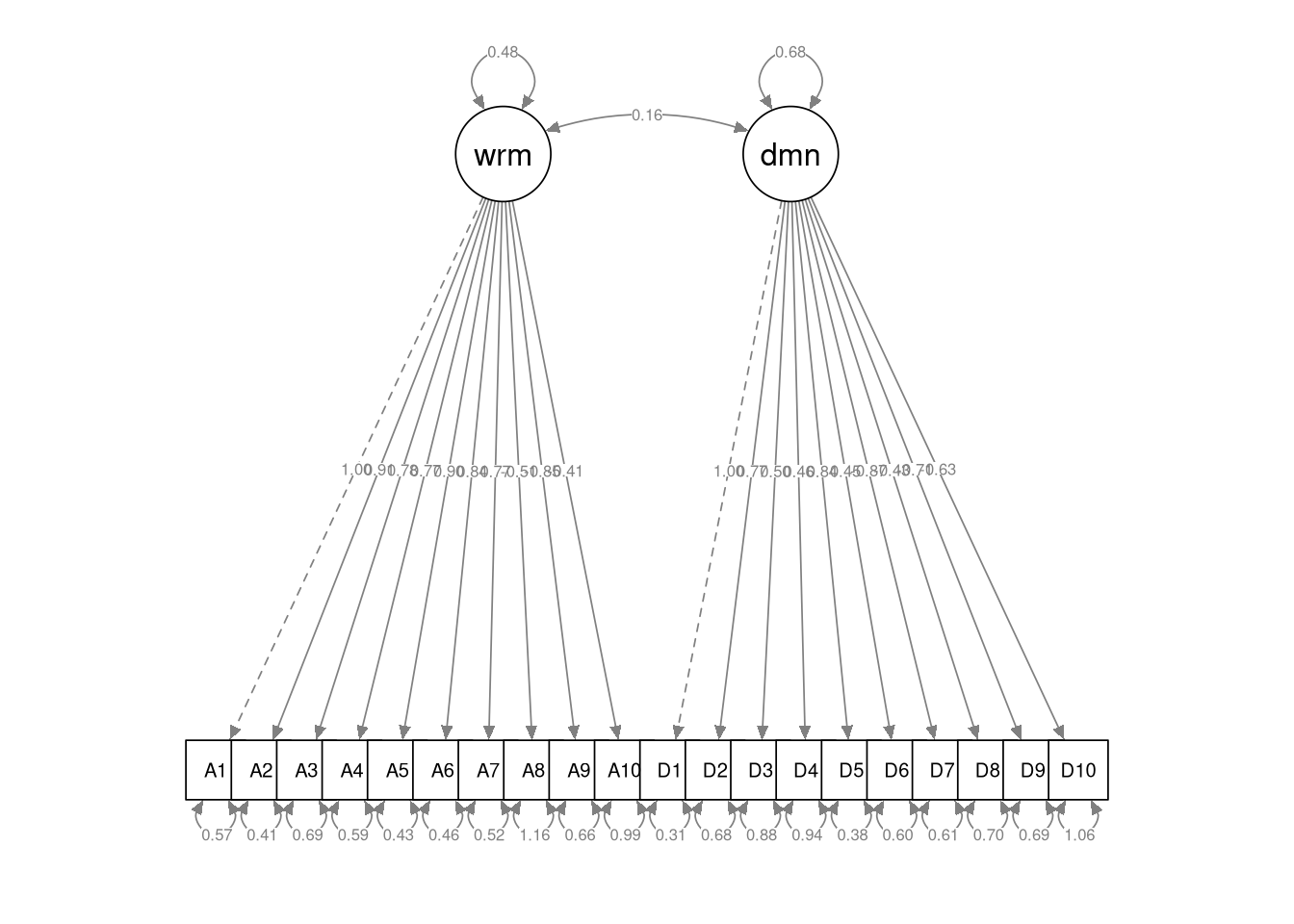
## warmth ~~
## dominance 0.156 0.023 6.920 0.000
##
## Variances:
## Estimate Std.Err z-value P(>|z|)
## .A1 0.567 0.030 18.988 0.000
## .A2 0.414 0.022 18.548 0.000
## .A3 0.689 0.033 20.683 0.000
## .A4 0.590 0.029 20.443 0.000
## .A5 0.428 0.023 18.734 0.000
## .A6 0.465 0.024 19.494 0.000
## .A7 0.518 0.026 20.166 0.000
## .A8 1.159 0.053 21.939 0.000
## .A9 0.659 0.032 20.288 0.000
## .A10 0.994 0.045 22.035 0.000
## .D1 0.307 0.021 14.578 0.000
## .D2 0.677 0.033 20.272 0.000
## .D3 0.877 0.040 21.695 0.000
## .D4 0.935 0.043 21.827 0.000
## .D5 0.376 0.021 17.825 0.000
## .D6 0.602 0.028 21.576 0.000
## .D7 0.606 0.031 19.352 0.000
## .D8 0.696 0.032 21.750 0.000
## .D9 0.689 0.033 20.626 0.000
## .D10 1.064 0.050 21.486 0.000
## warmth 0.480 0.042 11.314 0.000
## dominance 0.677 0.045 15.133 0.0004.3.12
Report the following parameter estimates from the model you estimated in 4.3.11.
- The
warmth\(\rightarrow\)A3factor loading - The
dominance\(\rightarrow\)D2factor loading - The latent covariance between warmth and dominance
Click to show answer
- \(\lambda_{3,1} = 0.78\)
- \(\lambda_{12,2} = 0.774\)
- \(\psi_{2,1} = 0.156\)
4.3.13
Based on the CFA you estimated in 4.3.11, can we infer a significant linear association between Warmth and Dominance?
- Use the statistics from your estimated model to justify your conclusion.
Click to show answer
Yes, warmth and dominance are significantly correlated (\(\psi_{2,1} = 0.156\), \(SE = 0.02\), \(z = 6.92\), \(p < 0.001\)).
4.3.14
Use the semPaths() function to draw a path diagram of your estimated CFA.
- Include the parameter estimates in the diagram.
4.3.15
Estimate a modified version of the two-factor CFA from 4.3.11, and summarize the results.
- Estimate the mean structure.
- Identify the model with the fixed factor method (i.e., standardize the latent variables).
Click to show code
## lavaan 0.6-19 ended normally after 18 iterations
##
## Estimator ML
## Optimization method NLMINB
## Number of model parameters 61
##
## Number of observations 1000
##
## Model Test User Model:
##
## Test statistic 1158.738
## Degrees of freedom 169
## P-value (Chi-square) 0.000
##
## Parameter Estimates:
##
## Standard errors Standard
## Information Expected
## Information saturated (h1) model Structured
##
## Latent Variables:
## Estimate Std.Err z-value P(>|z|)
## warmth =~
## A1 0.692 0.031 22.629 0.000
## A2 0.629 0.027 23.601 0.000
## A3 0.540 0.031 17.309 0.000
## A4 0.534 0.029 18.281 0.000
## A5 0.624 0.027 23.203 0.000
## A6 0.578 0.027 21.349 0.000
## A7 0.535 0.028 19.290 0.000
## A8 -0.352 0.038 -9.296 0.000
## A9 -0.586 0.031 -18.859 0.000
## A10 -0.286 0.035 -8.216 0.000
## dominance =~
## D1 0.823 0.027 30.267 0.000
## D2 0.636 0.032 20.101 0.000
## D3 0.411 0.033 12.379 0.000
## D4 0.380 0.034 11.178 0.000
## D5 0.692 0.026 26.161 0.000
## D6 0.370 0.028 13.335 0.000
## D7 -0.720 0.031 -22.953 0.000
## D8 -0.351 0.029 -11.894 0.000
## D9 -0.586 0.031 -18.697 0.000
## D10 -0.519 0.037 -13.994 0.000
##
## Covariances:
## Estimate Std.Err z-value P(>|z|)
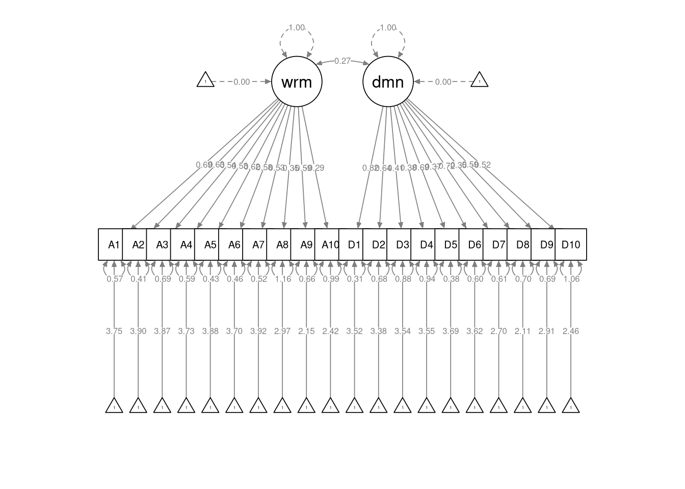
## warmth ~~
## dominance 0.273 0.035 7.906 0.000
##
## Intercepts:
## Estimate Std.Err z-value P(>|z|)
## .A1 3.748 0.032 115.859 0.000
## .A2 3.895 0.028 136.858 0.000
## .A3 3.865 0.031 123.414 0.000
## .A4 3.726 0.030 125.967 0.000
## .A5 3.876 0.029 135.635 0.000
## .A6 3.701 0.028 130.883 0.000
## .A7 3.919 0.028 138.175 0.000
## .A8 2.973 0.036 83.024 0.000
## .A9 2.146 0.032 67.772 0.000
## .A10 2.423 0.033 73.864 0.000
## .D1 3.522 0.031 112.305 0.000
## .D2 3.383 0.033 102.831 0.000
## .D3 3.545 0.032 109.611 0.000
## .D4 3.548 0.033 107.977 0.000
## .D5 3.686 0.029 126.029 0.000
## .D6 3.618 0.027 133.174 0.000
## .D7 2.701 0.034 80.578 0.000
## .D8 2.111 0.029 73.779 0.000
## .D9 2.910 0.032 90.589 0.000
## .D10 2.462 0.037 67.444 0.000
##
## Variances:
## Estimate Std.Err z-value P(>|z|)
## .A1 0.567 0.030 18.988 0.000
## .A2 0.414 0.022 18.548 0.000
## .A3 0.689 0.033 20.683 0.000
## .A4 0.590 0.029 20.443 0.000
## .A5 0.428 0.023 18.734 0.000
## .A6 0.465 0.024 19.494 0.000
## .A7 0.518 0.026 20.166 0.000
## .A8 1.159 0.053 21.939 0.000
## .A9 0.659 0.032 20.288 0.000
## .A10 0.994 0.045 22.035 0.000
## .D1 0.307 0.021 14.578 0.000
## .D2 0.677 0.033 20.272 0.000
## .D3 0.877 0.040 21.695 0.000
## .D4 0.935 0.043 21.827 0.000
## .D5 0.376 0.021 17.825 0.000
## .D6 0.602 0.028 21.576 0.000
## .D7 0.606 0.031 19.352 0.000
## .D8 0.696 0.032 21.750 0.000
## .D9 0.689 0.033 20.626 0.000
## .D10 1.064 0.050 21.486 0.000
## warmth 1.000
## dominance 1.0004.3.16
Report the following parameter estimates from the model you estimated in 4.3.15.
- The item intercept for
A1 - The item intercept for
D5 - The mean of the Warmth factor
Click to show answer
- \(\tau_1 = 3.75\)
- \(\tau_{15} = 3.69\)
- This is a bit of a trick question. We fixed the latent means to zero for model identification, so we don’t have an estimated latent mean for the warmth factor.
4.3.17
Based on the CFA you estimated in 4.3.15, how strong is the association between Warmth and Dominance?
- Use the statistics from your estimated model to justify your conclusion.
Click to show answer
We set the scale by standardizing the latent factors, so we can interpret the latent covariance as a correlation. Hence, the estimated latent covariance of \(\psi_{2,1} = 0.273\) suggests a weak linear association between Warmth and Dominance.
4.3.18
Use the semPaths() function to draw a path diagram of the CFA you estimated in 4.3.15.
- Include the parameter estimates in the diagram.
End of At-Home Exercises